

Growth model of the reared sea urchin Paracentrotus ... - SciViews
Growth model of the reared sea urchin Paracentrotus ... - SciViews
Growth model of the reared sea urchin Paracentrotus ... - SciViews

You also want an ePaper? Increase the reach of your titles
YUMPU automatically turns print PDFs into web optimized ePapers that Google loves.
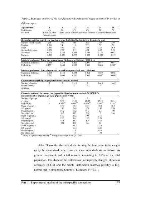
Table 7. Statistical analysis <strong>of</strong> <strong>the</strong> size frequency distribution <strong>of</strong> single cohorts <strong>of</strong> P. lividus at<br />
different ages.<br />
Age (months) 1 6 12 18 24 30<br />
Fertilization Fa Fb Fb Fb Fb Fb<br />
treatment Killed 7d. after<br />
metamorphosis<br />
Same cohort <strong>of</strong> <strong>reared</strong> echinoids followed in controlled conditions<br />
General descriptive statistics on size frequencies (individual horizontal test diameter in mm)<br />
Number <strong>of</strong> individuals 296 536 361 296 285 280<br />
Median 0.501 4 15 23 31 36<br />
Mean 0.497 4.81 17.1 24.6 32.3 36.9<br />
Standard deviation 0.056 2.28 5.51 6.98 6.12 5.56<br />
Skewness -0.275 0.748 0.851 0.599 0.136 0.042<br />
Kurtosis 0.226 -0.044 0.373 0.094 -0.024 0.139<br />
Intrinsic goodness <strong>of</strong> fit test to a normal curve (Kolmogorov-Smirnov / Lilliefors)<br />
Maximum difference 0.046 0.172 0.125 0.097 0.077 0.064<br />
Probability 0.127 **<br />
0.000 0.000 0.000 0.000 0.011 *<br />
Intrinsic goodness <strong>of</strong> fit to a log-normal curve (Kolmogorov-Smirnov / Lilliefors)<br />
Maximum difference 0.068 0.130 0.075 0.064 0.059 0.095<br />
Probability 0.002 0.000 0.000 0.005 0.018 *<br />
0.000<br />
Components analysis by <strong>the</strong> graphical Bhattacharya's method<br />
Number <strong>of</strong> modes 1 2 3 or 4 2 3 or 4 1 or 2<br />
Groups clearly<br />
separated<br />
- - 2 2 2 -<br />
Characterization <strong>of</strong> <strong>the</strong> groups (maximum-likelihood estimator method, NORMSEP)<br />
(minimal number <strong>of</strong> groups giving a χ 2 probability > 0.05)<br />
Number <strong>of</strong> groups - 2 3 2 3 1<br />
χ 2 value - 8.41 14.50 21.44 24.48 26.71<br />
Probability - 0.077 **<br />
0.488 **<br />
0.554 **<br />
Part III: Experimental studies <strong>of</strong> <strong>the</strong> intraspecific competition<br />
0.140 **<br />
0.181 **<br />
Mean <strong>of</strong> group 1 3.43 13.3 23.1 18.4 36.9<br />
SD group 1 1.15 2.49 5.39 1.82 5.56<br />
Percentage in 1 58.2 53.2 91.3 2.3 100<br />
No. <strong>of</strong> ind. in 1 312 192 269 7 280<br />
Mean <strong>of</strong> group 2 6.73 20.2 39.6 27.7<br />
SD group 2 2.07 3.61 1.97 2.54<br />
Percentage in 2 41.8 41.7 8.7 34.4<br />
No. <strong>of</strong> ind. in 2 224 151 26 98<br />
Mean <strong>of</strong> group 3 31.2 35.3<br />
SD group 3 1.34 5.00<br />
Percentage in 3 5.1 63.3<br />
No. <strong>of</strong> ind. in 3 18 179<br />
* Fitting is significant (p > 0.01); ** Fitting is very significant (p > 0.05).<br />
After 24 months, <strong>the</strong> individuals forming <strong>the</strong> head seem to be caught<br />
up by <strong>the</strong> mean sized ones. However, some individuals do not follow this<br />
general movement, and a tail remains amounting to 2.7% <strong>of</strong> <strong>the</strong> total<br />
population. The shape <strong>of</strong> <strong>the</strong> distribution is completely changed: skewness<br />
decreases (0.136) and <strong>the</strong> whole distribution matches possibly a lognormal<br />
one (Kolmogorov-Smirnov / Lilliefors, p > 0.01).<br />
119