Pre-Phase A Report - Lisa - Nasa

106 Chapter 4 Measurement Sensitivity
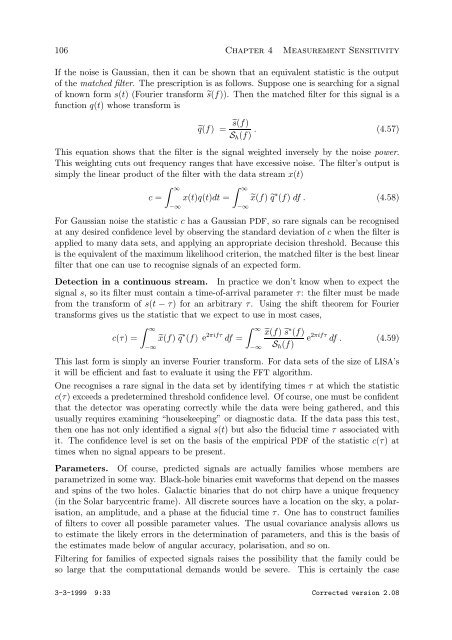
If the noise is Gaussian, then it can be shown that an equivalent statistic is the output
of the matched filter. The prescription is as follows. Suppose one is searching for a signal
of known form s(t) (Fourier transform s(f)). Then the matched filter for this signal is a
function q(t) whose transform is
q(f) = s(f)
. (4.57)
Sh(f)
This equation shows that the filter is the signal weighted inversely by the noise power.
This weighting cuts out frequency ranges that have excessive noise. The filter’s output is
simply the linear product of the filter with the data stream x(t)
c =
∞
−∞
x(t)q(t)dt =
∞
−∞
x(f) q ∗ (f) df . (4.58)
For Gaussian noise the statistic c has a Gaussian PDF, so rare signals can be recognised
at any desired confidence level by observing the standard deviation of c when the filter is
applied to many data sets, and applying an appropriate decision threshold. Because this
is the equivalent of the maximum likelihood criterion, the matched filter is the best linear
filter that one can use to recognise signals of an expected form.
Detection in a continuous stream. In practice we don’t know when to expect the
signal s, so its filter must contain a time-of-arrival parameter τ: the filter must be made
from the transform of s(t − τ) for an arbitrary τ. Using the shift theorem for Fourier
transforms gives us the statistic that we expect to use in most cases,
∞
c(τ) = x(f) q ∗ (f) e2πifτ ∞
df =
x(f) s ∗ (f)
e
Sh(f)
2πifτ df . (4.59)
−∞
This last form is simply an inverse Fourier transform. For data sets of the size of LISA’s
it will be efficient and fast to evaluate it using the FFT algorithm.
One recognises a rare signal in the data set by identifying times τ at which the statistic
c(τ) exceeds a predetermined threshold confidence level. Of course, one must be confident
that the detector was operating correctly while the data were being gathered, and this
usually requires examining “housekeeping” or diagnostic data. If the data pass this test,
then one has not only identified a signal s(t) but also the fiducial time τ associated with
it. The confidence level is set on the basis of the empirical PDF of the statistic c(τ) at
times when no signal appears to be present.
Parameters. Of course, predicted signals are actually families whose members are
parametrized in some way. Black-hole binaries emit waveforms that depend on the masses
and spins of the two holes. Galactic binaries that do not chirp have a unique frequency
(in the Solar barycentric frame). All discrete sources have a location on the sky, a polarisation,
an amplitude, and a phase at the fiducial time τ. One has to construct families
of filters to cover all possible parameter values. The usual covariance analysis allows us
to estimate the likely errors in the determination of parameters, and this is the basis of
the estimates made below of angular accuracy, polarisation, and so on.
Filtering for families of expected signals raises the possibility that the family could be
so large that the computational demands would be severe. This is certainly the case
3-3-1999 9:33 Corrected version 2.08
−∞