Pre-Phase A Report - Lisa - Nasa

112 Chapter 4 Measurement Sensitivity
as operating effectively like a pair of two-arm interferometers that measure orthogonal
polarisations.
How is the noise in interferometer I correlated with that in interferometer II ? This has
not yet been analyzed in detail. However one can show that if the detector noise in the
three individual arms is totally symmetric (so that all three arms have the same rms
noise amplitude, and the correlation between any pair of arms is also the same), then
the noise correlations between interferometers I and II exactly cancel out; they can be
regarded as statistically independent detectors [113]. As a first approximation, then, we
treat the noises in interferometers I and II as uncorrelated. It seems unlikely that a small
correlation between them would significantly affect the results presented below.
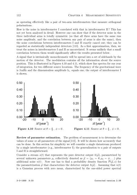
A signal that is intrinsically monochromatic will be spread into a set of sidebands by the
motion of the detector. The modulation contains all the information about the source
position. This is illustrated in Figures 4.10 and 4.11, which show line spectra for one year
of integration, for two different source locations. The frequency of the gravitational wave
is 3 mHz and the dimensionless amplitude h+ equals one; the output of interferometer I
is shown.
0.50
0.40
0.30
0.20
0.10
-20 -10 0
Δf [year
10 20
-1
0.00
]
Figure 4.10 Source at θ = π
2 ,φ=0.
0.50
0.40
0.30
0.20
0.10
-20 -10 0
Δf [year
10 20
-1
0.00
]
Figure 4.11 Source at θ = π
4 ,φ=0.
Review of parameter estimation. The problem of measurement is to determine the
values of some or all parameters of the signal [115]. It will be shown how accurately that
can be done. In this section for simplicity we will consider a single datastream produced
by a single interferometer (e.g., interferometer I); the generalization to a pair of outputs
I and II is straightforward.
Consider a stream s(t) that represents the pure detector output h(µ), parametrized by
several unknown parameters µi collectively denoted as µ =(µ1 = θ, µ2 = φ,...)plus
additional noise n(t) . Now one has to find a probability density function P(µ, s) for
the parametrization µ that characterizes the detector output h(µ) . Assuming that n(t)
is a Gaussian process with zero mean, characterized by the one-sided power spectral
3-3-1999 9:33 Corrected version 2.08