- Page 1 and 2:
ECOLOGY, BEHAVIOR & CONSERVATION OF
- Page 3 and 4:
discomfort without proper protectio
- Page 5 and 6:
ABOUT BELIZE Research Site: The pro
- Page 7 and 8:
FIELD TRAINING AND ASSIGNMENTS Duri
- Page 9 and 10:
ENVIRONMENTAL CONDITIONS SBCRC is s
- Page 11 and 12:
HEALTH INFORMATION Routine Immuniza
- Page 13 and 14:
• Consult the CDC for immunizatio
- Page 15 and 16:
Oil or oil-based repellant (e.g. ol
- Page 17 and 18:
Ecology, Behavior, and Conservation
- Page 19 and 20:
MINIMUM / MAXIMUM CLASS SIZE: 6-24
- Page 21 and 22:
COURSE FEE & ADDITIONAL INFORMATION
- Page 23 and 24:
Ecology, Behavior & Conservation of
- Page 25 and 26:
2012 Field Course Policy & Liabilit
- Page 27 and 28:
2012 Field Course Policy & Liabilit
- Page 29 and 30:
FIELD JOURNALS You are required to
- Page 31 and 32:
OUR INVESTIGATION Figure 2. G. crut
- Page 33 and 34:
OUR INVESTIGATION Introduction The
- Page 35 and 36:
OUR INVESTIGATION Introduction On a
- Page 37 and 38:
Method We selected a patch reef loc
- Page 39 and 40:
139 140 141 142 143 144 145 146 147
- Page 41 and 42:
OUR INVESTIGATION Introduction We f
- Page 43 and 44:
OUR RESEARCH FINDINGS Introduction
- Page 45 and 46:
area on the north part of the islan
- Page 47 and 48:
Introduction Our Investigation Befo
- Page 49 and 50:
Introduction Sea stars have long be
- Page 51 and 52:
INVESTIGATION Introduction Retracti
- Page 53 and 54:
Introduction Shells serve as a limi
- Page 55 and 56:
Introduction Lunar reproductive rhy
- Page 57 and 58:
TRIP SUMMARY SHEET (page 1) Day of
- Page 59 and 60:
RECORD OF EFFORT DATA SHEET Event (
- Page 61 and 62:
MANATEE SIGHTINGS AND SCANS Page 2
- Page 63 and 64:
MANATEE SIGHTINGS AND SCANS Page 4
- Page 65 and 66:
Date: Page 2 of ____ Sight/Scan Rec
- Page 67 and 68:
Date: Page 4 of ____ Sight/Scan Rec
- Page 69 and 70:
Sighting Log Continued from Page 1
- Page 71 and 72:
2010 VT: Scholar, BANNER, Safe Zone
- Page 73 and 74:
presentation to Horn Point Environm
- Page 75 and 76:
• Developed and managed education
- Page 77 and 78:
LaCommare, Katherine S. November 20
- Page 79 and 80:
• Comparative Vertebrate Anatomy,
- Page 81 and 82:
B. Ouranos, C. Bursey, and H. Kalb.
- Page 83 and 84:
2006. Holy Redeemer Day Camp. Conta
- Page 85 and 86:
18 NEWS AND VIEWS By 1995, in respo
- Page 87 and 88:
4842 J. M. BLUMENTHAL ET AL. are co
- Page 89 and 90:
4844 J. M. BLUMENTHAL ET AL. templa
- Page 91 and 92:
4846 J. M. BLUMENTHAL ET AL. Fig. 2
- Page 93 and 94:
4848 J. M. BLUMENTHAL ET AL. Fig. 4
- Page 95 and 96:
4850 J. M. BLUMENTHAL ET AL. mixed
- Page 97 and 98:
4852 J. M. BLUMENTHAL ET AL. Formia
- Page 99 and 100:
The Elusive Manatee -- An ethologic
- Page 101 and 102:
during the summer months while othe
- Page 103 and 104:
polyandrous - often mating with sev
- Page 105 and 106:
in the summer. Chessie, a male Flor
- Page 107 and 108:
ecords indicate that manatees have
- Page 109 and 110:
Florida manatee. National Biologica
- Page 111 and 112:
parturition: the action or process
- Page 113 and 114:
Manatees on the Belize Barrier Reef
- Page 115 and 116:
(a) (b) Manatees on the Belize Barr
- Page 117 and 118:
direction, and (e) when ‘travelli
- Page 119 and 120:
Season signi cantly aVected mean se
- Page 121 and 122:
male travelled at least as far as B
- Page 123 and 124:
55. Ontario Fisheries Research Labo
- Page 125 and 126:
NEWS OF THE WEEK MEETINGBRIEFS>> 10
- Page 127 and 128:
Functional Ecology 2008, 22, 284-28
- Page 129 and 130:
286 S. R. Noren Fig. 3. Swimming ki
- Page 131 and 132:
288 S. R. Noren Kelly, H.R. (1959)
- Page 133 and 134:
630 MARINE MAMMAL SCIENCE, VOL. 23,
- Page 135 and 136:
632 MARINE MAMMAL SCIENCE, VOL. 23,
- Page 137 and 138:
634 MARINE MAMMAL SCIENCE, VOL. 23,
- Page 139 and 140:
636 MARINE MAMMAL SCIENCE, VOL. 23,
- Page 141 and 142:
638 MARINE MAMMAL SCIENCE, VOL. 23,
- Page 143 and 144:
640 MARINE MAMMAL SCIENCE, VOL. 23,
- Page 145 and 146:
642 MARINE MAMMAL SCIENCE, VOL. 23,
- Page 147 and 148:
644 MARINE MAMMAL SCIENCE, VOL. 23,
- Page 149 and 150:
646 MARINE MAMMAL SCIENCE, VOL. 23,
- Page 151 and 152:
648 MARINE MAMMAL SCIENCE, VOL. 23,
- Page 153 and 154:
MARINE MAMMAL SCIENCE, 15(1): 102-1
- Page 155 and 156:
104 MARINE MAMMAL SCIENCE, VOL. 15.
- Page 157 and 158:
106 MARINE MAMMAL SCIENCE, VOL. 15,
- Page 159 and 160:
108 MARINE MAMMAL SCIENCE, VOL. 15,
- Page 161 and 162:
110 MARINE MAMMAL SCIENCE, VOL. 15,
- Page 163 and 164:
112 MARINE MAMMAL SCIENCE, VOL. 15,
- Page 165 and 166:
114 MARINE MAMMAL SCIENCE. VOL. 15.
- Page 167 and 168:
116 MARINE MAMMAL SCIENCE, VOL. 15,
- Page 169 and 170:
118 MARINE MAMMAL SCIENCE. VOL. 15.
- Page 171 and 172:
120 MARINE MAMMAL SCIENCE, VOL. 15,
- Page 173 and 174:
122 MARINE MAMMAL SCIENCE, VOL. 15,
- Page 175 and 176:
36 LaCommare et al. to the Drowned
- Page 177 and 178:
38 LaCommare et al. Figure 2. Map o
- Page 179 and 180:
40 LaCommare et al. points was 0.31
- Page 181 and 182:
42 LaCommare et al. may even provid
- Page 183 and 184:
172 NOTES Caribbean Journal of Scie
- Page 185 and 186:
174 FIG. 1. Drowned Cayes study are
- Page 187 and 188:
176 severe event occurred in 1998 (
- Page 189 and 190:
Coral Reefs (1997) 16, Suppl.: S23
- Page 191 and 192:
Table 1. Caribbean Diadema lore Sou
- Page 193 and 194:
Table 2. Historical accounts of the
- Page 195 and 196:
Table 3. Excerpts from Ernest F. Th
- Page 197 and 198:
Bradbury RH, Seymour RM, Antonelli
- Page 199 and 200:
Social Interactions in Captive Fema
- Page 201 and 202:
Captive Female Manatee Social Behav
- Page 203 and 204:
Captive Female Manatee Social Behav
- Page 205 and 206:
Captive Female Manatee Social Behav
- Page 207 and 208:
ut not random. Behaviors were not o
- Page 209 and 210:
Community Structure, Population Con
- Page 211 and 212:
422 THE AMERICAN NATURALIST the pla
- Page 213 and 214:
424 THE AMERICAN NATURALIST sarily
- Page 220 and 221:
Environmental Conservation 29 (2):
- Page 222 and 223:
194 C.M. Duarte well as more recent
- Page 224 and 225:
196 C.M. Duarte atmospheric inputs
- Page 226 and 227:
198 C.M. Duarte development (Short
- Page 228 and 229:
200 C.M. Duarte POTENTIAL STATUS IN
- Page 230 and 231:
202 C.M. Duarte detecting losses of
- Page 232 and 233:
204 C.M. Duarte Coles, R. & Fortes,
- Page 234 and 235:
206 C.M. Duarte Ramos-Esplá, A., M
- Page 236 and 237:
$1.2 million (Moore et al. 2009a).
- Page 238 and 239:
and positively related to knowledge
- Page 240 and 241:
student’s ability to learn facts
- Page 242 and 243:
Conservation and Behaviour Richard
- Page 244 and 245:
animals may adopt microhabitat choi
- Page 246 and 247:
and minimize traffic-induced wildli
- Page 248 and 249:
decision rules they use in response
- Page 250 and 251:
Gagnon JW, Theimer TC, Dodd NL, Boe
- Page 252 and 253:
402 Opinion TRENDS in Ecology and E
- Page 254 and 255:
404 Opinion TRENDS in Ecology and E
- Page 256 and 257:
406 Opinion TRENDS in Ecology and E
- Page 258 and 259:
Anim Cogn (2009) 12:43-53 DOI 10.10
- Page 260 and 261:
Anim Cogn (2009) 12:43-53 45 Fig. 1
- Page 262 and 263:
Anim Cogn (2009) 12:43-53 47 Table
- Page 264 and 265:
Anim Cogn (2009) 12:43-53 49 Table
- Page 266 and 267:
Anim Cogn (2009) 12:43-53 51 the pr
- Page 268 and 269:
Anim Cogn (2009) 12:43-53 53 L, Rei
- Page 270 and 271:
(Halodule wrightii and Syringodium
- Page 272 and 273:
Diurnal and Nocturnal Scans Four of
- Page 274 and 275:
Figure 3. The number of scans (whit
- Page 276 and 277:
in 2006. Although this difference i
- Page 278 and 279:
manatus in Costa Rica. Biological C
- Page 280 and 281:
574 D. J. Semeyn et al. and natural
- Page 282 and 283: 576 D. J. Semeyn et al. Fig. 1 Refe
- Page 284 and 285: 578 D. J. Semeyn et al. Fig. 3 Refe
- Page 286 and 287: 580 D. J. Semeyn et al. Fig. 4 Kern
- Page 288 and 289: 582 D. J. Semeyn et al. biologists
- Page 290 and 291: Intraspecific and geographic variat
- Page 292 and 293: III. RESULTS Manatees in Florida an
- Page 294 and 295: Genetica (2011) 139:833-842 DOI 10.
- Page 296 and 297: Genetica (2011) 139:833-842 835 dur
- Page 298 and 299: Genetica (2011) 139:833-842 837 Tab
- Page 300 and 301: Genetica (2011) 139:833-842 839 Man
- Page 302 and 303: Genetica (2011) 139:833-842 841 edu
- Page 304 and 305: Fish Sci (2011) 77:795-798 DOI 10.1
- Page 306 and 307: Fish Sci (2011) 77:795-798 797 was
- Page 308 and 309: Low genetic variation and evidence
- Page 310 and 311: Reduced Belize manatee dispersal an
- Page 312 and 313: Reduced Belize manatee dispersal an
- Page 314 and 315: Reduced Belize manatee dispersal an
- Page 316 and 317: Reduced Belize manatee dispersal an
- Page 318 and 319: Reduced Belize manatee dispersal an
- Page 320 and 321: and respond to human encounters by
- Page 322 and 323: tourist vessels are present, and th
- Page 324 and 325: that approach behaviour may be habi
- Page 326 and 327: to structure almost completely the
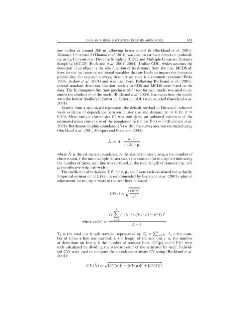
- Page 328 and 329: MARINE MAMMAL SCIENCE, 27(3): 606-6
- Page 330 and 331: 608 MARINE MAMMAL SCIENCE, VOL. 27,
- Page 334 and 335: 612 MARINE MAMMAL SCIENCE, VOL. 27,
- Page 336 and 337: 614 MARINE MAMMAL SCIENCE, VOL. 27,
- Page 338 and 339: 616 MARINE MAMMAL SCIENCE, VOL. 27,
- Page 340 and 341: 618 MARINE MAMMAL SCIENCE, VOL. 27,
- Page 342 and 343: 620 MARINE MAMMAL SCIENCE, VOL. 27,
- Page 344 and 345: Journal of Zoology The lesser of tw
- Page 346 and 347: E. M. Arraut et al. & Sparks, 1989)
- Page 348 and 349: E. M. Arraut et al. Frequent cloud
- Page 350 and 351: E. M. Arraut et al. rising-water we
- Page 352 and 353: E. M. Arraut et al. (Link, 1795) an
- Page 354 and 355: The Journal of Experimental Biology
- Page 356 and 357: Fig. 1. Rescue locations of manatee
- Page 358 and 359: The present study is the first to c
- Page 360 and 361: Bearhop, S., Waldron, S., Votier, S
- Page 362 and 363: 1
2
3
4
5
6
7
- Page 364 and 365: 46
47
48
49
50
51
- Page 366 and 367: 89
90
91
92
93
94
- Page 368 and 369: 134
135
136
137
138
- Page 370 and 371: 176
177
178
179
180
- Page 372 and 373: 218
219
220
221
222
- Page 374 and 375: 262
263
264
265
266
- Page 376 and 377: 308
309
310
311
312
- Page 378 and 379: 354
355
356
357
358
- Page 380 and 381: 402
403
404
405
406
- Page 382 and 383:
436
437
438
439
440
- Page 384 and 385:
494
495
496
497
498
- Page 386 and 387:
Table 1. Results from the GLM relat
- Page 388 and 389:
28
- Page 390 and 391:
Figure 1. Map of the Drowned Cayes
- Page 392 and 393:
Figure 3. Histogram of number of ma
- Page 394 and 395:
a. b. c. Power Power Power 100 80 6