Equality, Participation, Transition: Essays in Honour of Branko Horvat
Equality, Participation, Transition: Essays in Honour of Branko Horvat
Equality, Participation, Transition: Essays in Honour of Branko Horvat

You also want an ePaper? Increase the reach of your titles
YUMPU automatically turns print PDFs into web optimized ePapers that Google loves.
58 Determ<strong>in</strong>ants <strong>of</strong> Income Inequality<br />
RESID<br />
20<br />
10<br />
0<br />
–10<br />
–20<br />
0 5000 10000 15000 20000<br />
PPP<br />
Figure 4.2 Residuals from equation 1.0 as a function <strong>of</strong> INCOME<br />
PPPGDP per capita <strong>in</strong> 1988 dollars <strong>of</strong> equal purchas<strong>in</strong>g power parity.<br />
RESIDresiduals from equation 1.0.<br />
which had become available s<strong>in</strong>ce the first draft <strong>of</strong> this study was<br />
completed. The De<strong>in</strong><strong>in</strong>ger–Squire data set is an unbalanced panel <strong>of</strong><br />
<strong>in</strong>equality measures for 101 countries cover<strong>in</strong>g the period from the<br />
1950s onward. Unfortunately for my purpose, it comb<strong>in</strong>es both<br />
<strong>in</strong>come and expenditure <strong>in</strong>equality measures: for a number <strong>of</strong> countries,<br />
only the distribution <strong>of</strong> expenditures is available. 18 For each <strong>of</strong> the<br />
80 countries <strong>in</strong> my sample, I have selected from the De<strong>in</strong><strong>in</strong>ger–Squire<br />
data base, the G<strong>in</strong>i coefficient and the qu<strong>in</strong>tile ratio 19 based on <strong>in</strong>come<br />
(or if unavailable, expenditures) from the mid-1980s. The sample size<br />
decl<strong>in</strong>es to 70 due to the fact that 10 countries from my data set are<br />
not <strong>in</strong>cluded <strong>in</strong> the De<strong>in</strong><strong>in</strong>ger–Squire set. Equation 1 is then rerun first,<br />
over the G<strong>in</strong>i coefficients from the De<strong>in</strong><strong>in</strong>ger–Squire data set (equation<br />
1A), and then over the qu<strong>in</strong>tile ratios from the same set (equation 1B).<br />
The signs <strong>of</strong> all the coefficients are the same as predicted and as <strong>in</strong><br />
equation 1. All coefficients except the one for TRANS rema<strong>in</strong> statistically<br />
highly significant, and their values (except for TRANS) change<br />
very little (compare, for example, equations 1 and 1A <strong>in</strong> Table 4.2). 20<br />
The R¯2 decreases from 0.7 to 0.42, and the constant term becomes<br />
significant at 5 per cent level. The results seem robust to the use <strong>of</strong>