Coherent Backscattering from Multiple Scattering Systems - KOPS ...

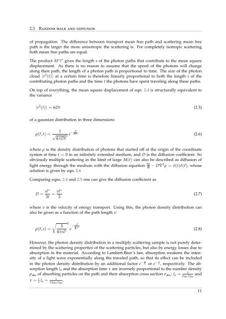
2.3 Random walk and diffusion
of propagation. The difference between transport mean free path and scattering mean free
path is the larger the more anisotropic the scattering is. For completely isotropic scattering
both mean free paths are equal.
The product M ∗ l ∗ gives the length s of the photon paths that contribute to the mean square
displacement. As there is no reason to assume that the speed of the photons will change
along their path, the length of a photon path is proportional to time. The size of the photon
cloud 〈r 2 (t)〉 at a certain time is therefore linearly proportional to both the length s of the
contributing photon paths and the time t the photons have spent traveling along these paths.
On top of everything, the mean square displacement of eqn. 2.4 is structurally equivalent to
the variance
〈r 2 (t)〉 = 6Dt (2.5)
of a gaussian distribution in three dimensions
ρ(⃗r, t) =
1
r2
√ e− 4Dt (2.6)
3
4πDt
where ρ is the density distribution of photons that started off at the origin of the coordinate
system at time t = 0 in an infinitely extended medium, and D is the diffusion coefficient. So
obviously multiple scattering in the limit of large M(t) can also be described as diffusion of
light energy through the medium with the diffusion equation ∂ρ
∂t − D∇2 ρ = δ(t)δ(⃗r), whose
solution is given by eqn. 2.6
Comparing eqns. 2.4 and 2.5 one can give the diffusion coefficient as
D = sl∗
3t = vl∗
3
(2.7)
where v is the velocity of energy transport. Using this, the photon density distribution can
also be given as a function of the path length s:
ρ(⃗r, s) =
√
3
4πsl ∗ 3
e − 4
r2
3 sl∗ (2.8)
However, the photon density distribution in a multiply scattering sample is not purely determined
by the scattering properties of the scattering particles, but also by energy losses due to
absorption in the material. According to Lambert-Beer’s law, absorption weakens the intensity
of a light wave exponentially along the traveled path, so that its effect can be included
in the photon density distribution by an additional factor e − la
s
or e − τ t , respectively. The absorption
length l a and the absorption time τ are inversely proportional to the number density
ρ abs of absorbing particles on the path and their absorption cross section σ abs : l a = 1
ρ abs σ abs
and
τ = t s l 1
a =
v ρ abs σ abs
.
11