Coherent Backscattering from Multiple Scattering Systems - KOPS ...

2 Theory
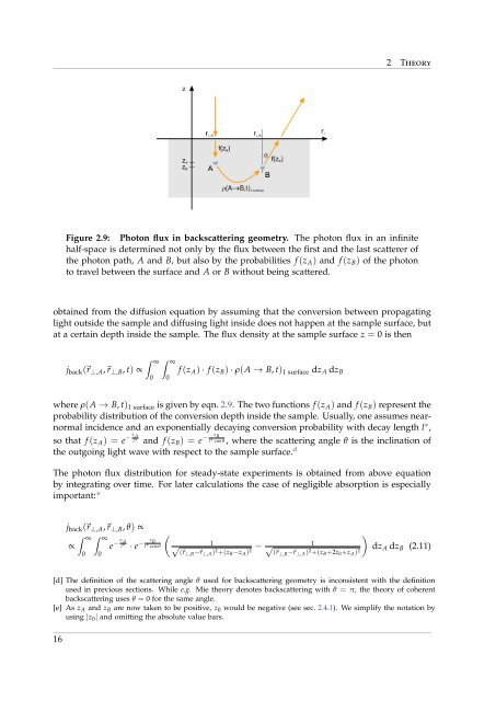
Figure 2.9: Photon flux in backscattering geometry. The photon flux in an infinite
half-space is determined not only by the flux between the first and the last scatterer of
the photon path, A and B, but also by the probabilities f (z A ) and f (z B ) of the photon
to travel between the surface and A or B without being scattered.
obtained from the diffusion equation by assuming that the conversion between propagating
light outside the sample and diffusing light inside does not happen at the sample surface, but
at a certain depth inside the sample. The flux density at the sample surface z = 0 is then
j back (⃗r ⊥,A ,⃗r ⊥,B , t) ∝
∫ ∞ ∫ ∞
0 0
f (z A ) · f (z B ) · ρ(A → B, t) 1 surface dz A dz B
where ρ(A → B, t) 1 surface is given by eqn. 2.9. The two functions f (z A ) and f (z B ) represent the
probability distribution of the conversion depth inside the sample. Usually, one assumes nearnormal
incidence and an exponentially decaying conversion probability with decay length l ∗ ,
so that f (z A ) = e − z A
l ∗
and f (z B ) = e − z B
l ∗ cos θ , where the scattering angle θ is the inclination of
the outgoing light wave with respect to the sample surface. d
The photon flux distribution for steady-state experiments is obtained from above equation
by integrating over time. For later calculations the case of negligible absorption is especially
important: e
j back (⃗r ⊥,A ,⃗r ⊥,B , θ) ∝
∝
∫ ∞ ∫ ∞
0
0
e − z A
l∗ · e − z B
l ∗ cos θ
(
)
√ 1
− √ 1
(⃗r⊥,B −⃗r ⊥,A ) 2 +(z B −z A ) 2 (⃗r⊥,B −⃗r ⊥,A ) 2 +(z B +2z 0 +z A ) 2
dz A dz B (2.11)
[d] The definition of the scattering angle θ used for backscattering geometry is inconsistent with the definition
used in previous sections. While e.g. Mie theory denotes backscattering with θ = π, the theory of coherent
backscattering uses θ = 0 for the same angle.
[e] As z A and z B are now taken to be positive, z 0 would be negative (see sec. 2.4.1). We simplify the notation by
using |z 0 | and omitting the absolute value bars.
16