Coherent Backscattering from Multiple Scattering Systems - KOPS ...

2 Theory
cooperon
1
0.8
0.6
0.4
l abs
= 10 −5 m
l abs
= 3 ⋅ 10 −5 m
l abs
= 10 −4 m
no absorption
0.2
0
−90 −60 −30 0 30 60 90
scattering angle [deg]
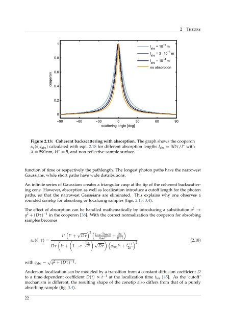
Figure 2.13: Coherent backscattering with absorption. The graph shows the cooperon
α c (θ, l abs ) calculated with eqn. 2.18 for different absorption lengths l abs = 3Dτ/l ∗ with
λ = 590 nm, kl ∗ = 5, and non-reflective sample surface.
function of time or respectively the pathlength. The longest photon paths have the narrowest
Gaussians, while short paths have wide distributions.
An infinite series of Gaussians creates a triangular cusp at the tip of the coherent backscattering
cone. However, absorption as well as localization introduce a cutoff length for the photon
paths, so that the narrowest Gaussians are eliminated. This explains why one observes a
rounded conetip for absorbing or localizing samples (figs. 2.13, 3.4).
The effect of absorption can be handled mathematically by introducing a substitution q 2 →
q 2 + (Dτ) −1 in the cooperon [38]. With the correct normalization the cooperon for absorbing
samples becomes
α c (θ, τ) =
(
Dτ l ∗ +
(
l ∗ l ∗ + √ ) 2 (
Dτ 1−e
−2q abs z 0
(
1 − e − 2z 0
q abs l ∗ + 2µ
µ+1
)
) )
√ √Dτ ( )
Dτ q abs l ∗ + µ+1 2
(2.18)
2µ
with q abs = √ q 2 + (Dτ) −1 .
Anderson localization can be modeled by a transition from a constant diffusion coefficient D
to a time-dependent coefficient D(t) ∝ t −1 at the localization time t loc [45]. As the ‘cutoff’
mechanism is different, the resulting shape of the conetip also differs from that of a purely
absorbing sample (fig. 3.4).
22