Coherent Backscattering from Multiple Scattering Systems - KOPS ...

5 Experiments
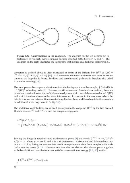
Figure 5.4: Contributions to the cooperon. The diagram on the left depicts the interference
of two light waves running on time-inverted paths between ⃗r 1 and ⃗r 2 . The
diagram on the right illustrates the light paths that include an additional scatterer in⃗r 0 .
cooperon as defined above is often expressed in terms of the Hikami box H (A) as I c (⃗r) ∝
∫∫ H (A) (⃗r 1 ,⃗r 2 ) · Γ(⃗r 1 ,⃗r 2 ) d⃗r 1 d⃗r 2 [25]. H (A) combines the four amplitudes that cross at the entrance
of the loop that is formed by direct and time-inverted path and is therefore also called
a quantum crossing [10].
The total power the cooperon distributes into the half-space above the sample, ∫ I c (θ) dΩ, is
∝ 1/(kl ∗ ) 2 in leading order [9]. However, as Akkermans and Montambaux realized, there are
two other contributions to the multiple scattered power which are of the same order in 1/(kl ∗ )
and which therefore also must be taken into account. In contrast to the cooperon, where the
interference occurs between time-inverted amplitudes, these additional contributions contain
an additional scattering event in⃗r 0 (fig. 5.4).
The additional contributions are defined analogous to the cooperon H (A) by the two dressed
Hikami boxes H (B) and H (C) , which are complex conjugates:
H (B) (⃗r,⃗ r ′ ,⃗r 1 ,⃗r 2 ) =
∫ 〈Ψin
= (⃗r,⃗r 1 ) 〉 · 〈Ψ
in(⃗r,⃗r ∗ 0 ) 〉 · 〈G ∗ (⃗r 0 ,⃗r 2 ) 〉 · 〈G(⃗r
2 ,⃗ r ′ ) 〉 · 〈G ∗ (⃗r 1 ,⃗r 0 ) 〉 · 〈G ∗ (⃗r 0 ,⃗ r ′ ) 〉 d⃗r 0
Solving the integrals requires some mathematical ploys [9] and yields I (B+C)
c ≈ −a/(kl ∗ ) 2 ·
µ/(µ + 1), where µ = cos θ, and a is a fit parameter. Akkermans and Montambaux obtain
a = 1.15 by fitting an intermediate result to experimental data from samples with wide
backscattering cones [9, 19]. However, one can also use the fact that the cooperon together
with the additional contributions now satisfies conservation of energy [8, 9, 10], so that
∫
I (A)
c
+ I (B+C)
c d(⃗r − ⃗ r ′ ) = 0
50