Coherent Backscattering from Multiple Scattering Systems - KOPS ...

4 Samples
4.1 Sample characterization techniques
The light scattering experiments performed with the setups introduced in sec. 3 are the main
source of data which characterize the multiple scattering samples. However, there are a few
additional sample properties which have to be obtained otherwise. These are mainly the
effective refractive index of the sample and the reflectivity of the sample surface, which are
necessary for example to calculate the average penetration depth z 0 . Also important are the
particle size and polydispersity of the samples and the filling fraction of the sample. Some
of these calculations are trivial and can be found in every physics textbook, but still are to be
mentioned briefly.
4.1.1 Particle size and polydispersity
Particle size and polydispersity of the the colloidal particles give first indications for the scattering
properties of the multiple scattering samples. Strongly scattering samples have particle
diameters of the order of the wavelength and low polydispersity. Especially strong scattering
is obtained when the scattering in the particles becomes resonant.
The commercial titanium dioxide samples have been characterized before by M. Störzer [47],
who used electron microscopy to determine size and polydispersity of the particles. The
device used was an XL Scanning Electron Microscope from Phillips, which provides a spatial
resolution of up to 50 nm. To avoid charge building in the sample the surface was covered with
a gold layer of approximately 10 nm thickness, which was brought onto the sample using a
gas discharge sputter technique (Scancoat SIX, Edwards). The distribution of the particle sizes
was obtained by measuring the diameters of 150-200 particles from the pictures (fig 4.1).
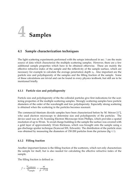
4.1.2 Filling fraction
Another important feature is the filling fraction of the scatterers, which not only characterizes
the sample for itself, but is also needed for calculating the effective refractive index of the
sample.
The filling fraction is defined as
f = V scatterers
V sample
=
m
ρ · r 2 πh