Coherent Backscattering from Multiple Scattering Systems - KOPS ...
Coherent Backscattering from Multiple Scattering Systems - KOPS ...
Coherent Backscattering from Multiple Scattering Systems - KOPS ...

You also want an ePaper? Increase the reach of your titles
YUMPU automatically turns print PDFs into web optimized ePapers that Google loves.
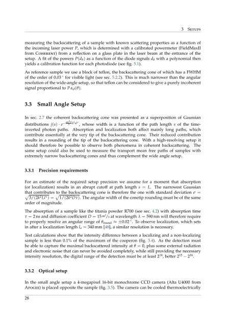
3 Setups<br />
measuring the backscattering of a sample with known scattering properties as a function of<br />
the incoming laser power P, which is determined with a calibrated powermeter (FieldMaxII<br />
<strong>from</strong> <strong>Coherent</strong>) <strong>from</strong> a reflection on a glass plate in the laser beam at the entrance of the<br />
setup. A fit of the powers P(d θ ) as a function of the diode signals d θ with a polynomial then<br />
yields a calibration function for each photodiode (see fig. 5.1).<br />
As reference sample we use a block of teflon, the backscattering cone of which has a FWHM<br />
of the order of 0.03 ◦ for visible light (see sec. 5.2.2). This is much narrower than the angular<br />
resolution of the wide-angle setup, so that teflon can be considered to give a purely incoherent<br />
signal proportional to P α d (θ).<br />
3.3 Small Angle Setup<br />
In sec. 2.7 the coherent backscattering cone was presented as a superposition of Gaussian<br />
distributions j(s) · e − sin2 θ<br />
3 k 2 sl ∗ , whose width is a function of the path length s of the timeinverted<br />
photon paths. Absorption and localization both affect mainly long paths, which<br />
contribute essentially at the very tip of the backscattering cone. Their reduced contribution<br />
results in a rounding of the tip of the backscattering cone. With a high-resolving setup it<br />
should therefore be possible to observe both phenomena in coherent backscattering. The<br />
same setup could also be used to measure the transport mean free paths of samples with<br />
extremely narrow backscattering cones and thus complement the wide angle setup.<br />
3.3.1 Precision requirements<br />
For an estimate of the required setup precision we assume for a moment that absorption<br />
(or localization) results in an abrupt cutoff at path length s = L. The narrowest Gaussian<br />
that contributes to the backscattering cone is therefore the one with standard deviation σ =<br />
√<br />
3/(2k 2 Ll ∗ ) = √ 1/(2k 2 Dτ). The angular width of the conetip rounding must be of the same<br />
order of magnitude.<br />
The absorption of a sample like the titania powder R700 (see sec. 4.2) with absorption time<br />
τ = 2 ns and diffusion coefficient D = 15 m2 /s at wavelength λ = 590 nm will therefore require<br />
to properly resolve an angular range of θ round ≈ ±0.02 ◦ . To observe localization, which sets<br />
in after a localization length l a = 340 mm [48], a similar resolution is necessary.<br />
Test calculations show that the intensity difference between a localizing and a non-localizing<br />
sample is less than 0.1% of the maximum of the cooperon (fig. 3.4). As the detection must<br />
be able to capture the maximal backscattered intensity at θ = 0, plus some external radiation<br />
and electronic noise that can never be avoided completely, while still providing the necessary<br />
intensity resolution, the digital range of the detection must be at least 2 14 , better 2 15 − 2 16 .<br />
3.3.2 Optical setup<br />
In the small angle setup a 4-megapixel 16-bit monochrome CCD camera (Alta U4000 <strong>from</strong><br />
Apogee) is placed opposite the sample (fig. 3.5). The camera can be cooled thermoelectrically<br />
28