Coherent Backscattering from Multiple Scattering Systems - KOPS ...

More documents

Recommendations

Info

5 Experiments space with the energy inside an absorbing cut-out of the half-space at the position of the sample: j with losses (⃗r ⊥ , t) = A(t) · j lossless (⃗r ⊥ , t) = j lossless (⃗r ⊥ , t) · ∫ ∫ finite sample infinite half-space ρ τ (⃗r, t) d⃗r ρ τ→∞ (⃗r, t) d⃗r This ignores the fact that the photon density distribution is altered by the sample boundaries, but if the sample is large enough, only a few photons reach those boundaries anyway, so that the presence of the boundaries is of nearly no consequence for the density distribution. As solving eqns. 5.5 and 5.3 for the photon density distribution of the infinite half-space raises considerable algebraic and numeric difficulties, we fall back to the density distribution in free space, where the solution is easier to obtain. Fig. 5.2 shows that the albedos A(t) are similar enough to make this assumption, although the actual photon density distributions look quite different (fig. 5.3). The only difference in the albedos occurs when the photon cloud reaches the boundaries, which for the teflon sample in the figure happens at photon travel times around 10 to 100 ns. Even at this point the error is only a few percent, which presumably is not larger than the error that is already made by ignoring the altered density distribution. (5.5) Evaluating eqn. 5.5 gives the albedo ∫ L 1 A(τ, L, R) = π(l ∗ +z 0 ) 0 (√ − K 0 K 0 (√ 4(l ∗ +z 0 ) 2 +z 2 Dτ z 2 Dτ ) − 2K 0 (√ ) + 2K 0 (√ ) (√ R 2 +z 2 Dτ + K 0 R 2 +4(l ∗ +z 0 ) 2 +z 2 Dτ ) − K 0 (√ ) 2R 2 +z 2 Dτ − 2R 2 +4(l ∗ +z 0 ) 2 +z 2 Dτ ) dz (5.6) where the K n (x) are modified Bessel functions of the second kind. The last step of integration is performed numerically. The transport mean free path l ∗ is the result of the evaluation of the backscattering data, for which the albedo is an input parameter. Therefore the correct value for l ∗ is not yet known when the albedo is calculated. Instead, we use l ∗ = 3D v ≈ 3n effD c 0 (see sec. 2.3), which should at least have the right order of magnitude. The resulting albedos for the samples examined in the backscattering experiments are given in tab. 5.1. One immediately observes the striking difference between the albedos of the titania samples, which are in excess of 99%, and the albedo of teflon, which is about 90%. The accuracy of the experiments therefore depends strongly on the accuracy of the teflon albedo. It is however nearly impossible to give an error for the calculated albedos, as the validity of the various assumptions is not known. Altogether, the error of the albedo mismatch is probably of the order of one or two percent. 5.1.3 The correct theory of coherent backscattering The first steps towards a theoretical description of coherent backscattering have already been taken in sec. 2.1, where the intensity in a multiple scattering medium is presented as the 48
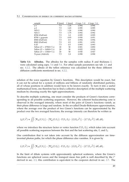
5.1 Conservation of energy in coherent backscattering sample R [mm] L [mm] A (eqn. 5.4) A (eqn. 5.6) a-1 7.5 1.35 0.994 0.994 a-2 7.5 1.03 0.995 0.995 NIX-2 7.5 1.26 0.990 0.990 NIX-3 7.5 1.75 0.992 0.992 R700 (DuPont) 7.5 1.0 0.995 0.995 R700 + gypsum 7.5 0.95 0.950 0.951 R900 (DuPont) 7.5 0.5 0.994 0.994 R902 (DuPont) 7.5 0.5 0.991 0.991 S-25 7.5 0.5 0.993 0.993 Teflon (D = 27500 m 2 /s) 20 50 0.901 0.890 Teflon (D = 16500 m 2 /s) 20 50 0.922 0.918 Teflon (D = 13300 m 2 /s) 20 50 0.930 0.927 Ti-pure (Aldrich) 7.5 1.8 0.998 0.998 Table 5.1: Albedos. The albedos for the samples with radius R and thickness L were calculated using eqns. 5.4 and 5.6. For other sample parameters see tab. 4.1 and sec. 4.2.2. The albedo of the teflon reference was calculated for the three different diffusion coefficients mentioned in sec. 4.2.2. solution of the wave equation by Green’s functions. This description would be exact, but it can not be solved for a system of millions and billions of randomly distributed particles, all of whose positions in addition would have to be known exactly. To turn it into a useful mathematical form, one therefore has to find a collective description of the multiple scattering medium by choosing exactly the right approximations. To describe multiple scattering, one must consider the products of Green’s functions corresponding to all possible scattering sequences. However, the coherent backscattering cone is observed in the averaged intensity, where most of the pairs of Green’s functions vanish, as their phase difference is large and random. In the so-called Drude-Boltzmann approximation, where the average over the product of two Green’s functions can be approximated by the product over the two averaged functions, the average intensity can therefore be written as ∫∫ 〈Ψin I d (⃗r,⃗ r ′ ) ∝ (⃗r,⃗r 1 ) 〉 · 〈Ψ in(⃗r,⃗r ∗ 1 ) 〉 · Γ(⃗r 1 ,⃗r 2 ) · 〈G(⃗r 2 ,⃗ r ′ ) 〉 · 〈G ∗ (⃗r 2 ,⃗ r ′ ) 〉 d⃗r 1 d⃗r 2 where we introduce the structure factor or vertex function Γ(⃗r 1 ,⃗r 2 ), which takes into account all possible scattering sequences between the first and the last scattering site,⃗r 1 and⃗r 2 . One contribution that is not taken into account by the diffuson approximation are timeinverted photon paths, for which the phase difference also vanishes. It is given by ∫∫ 〈Ψin I c (⃗r,⃗ r ′ ) ∝ (⃗r,⃗r 1 ) 〉 · 〈Ψ in(⃗r,⃗r ∗ 2 ) 〉 · Γ(⃗r 1 ,⃗r 2 ) · 〈G(⃗r 2 ,⃗ r ′ ) 〉 · 〈G ∗ (⃗r 1 ,⃗ r ′ ) 〉 d⃗r 1 d⃗r 2 In the limit of dilute systems with approximately spherical scatterers, where the Green’s functions are spherical waves and the transport mean free path is well described by the l ∗ derived in sec. 2.3, this contribution is equivalent to the cooperon derived in sec. 2.7. The 49
Page 1 and 2:
Dissertation Coherent Backscatterin
Page 3 and 4:
Ein kurzer Überblick Streuung ist
Page 5 and 6: Ein kurzer Überblick portweglänge
Page 7 and 8: Contents Ein kurzer Überblick i Da
Page 9 and 10: 1 Introduction There have been many
Page 11 and 12: 2 Theory In scattering theory, the
Page 13 and 14: 2.2 Single scattering - Mie theory
Page 15 and 16: 2.2 Single scattering - Mie theory
Page 17 and 18: 2.3 Random walk and diffusion scatt
Page 19 and 20: 2.3 Random walk and diffusion of pr
Page 21 and 22: 2.4 The influence of boundaries Fig
Page 23 and 24: 2.5 Photon flux from a surface The
Page 25 and 26: 2.6 On polarization and interferenc
Page 27 and 28: 2.6 On polarization and interferenc
Page 29 and 30: 2.7 The theory of coherent backscat
Page 31 and 32: 2.7 The theory of coherent backscat
Page 33 and 34: 3 Setups 3.1 Laser System The key p
Page 35 and 36: 3.2 Wide Angle Setup 1 .0 0 .8 h e
Page 37 and 38: 3.3 Small Angle Setup 1 0.998 0.996
Page 39 and 40: 3.3 Small Angle Setup Figure 3.6: T
Page 41 and 42: 3.4 Time Of Flight Setup Figure 3.8
Page 43 and 44: 4 Samples 4.1 Sample characterizati
Page 45 and 46: 4.1 Sample characterization techniq
Page 47 and 48: 4.2 The samples sample particle siz
Page 49 and 50: 4.2 The samples Figure 4.5: Fluidiz
Page 51 and 52: 5 Experiments 5.1 Conservation of e
Page 53 and 54: 5.1 Conservation of energy in coher
Page 55: 5.1 Conservation of energy in coher
Page 65 and 66: 5.2 The coherent backscattering con
Page 77 and 78: 6 Summary The focus of the work pre
Page 79 and 80: Bibliography [1] http://www.schneid
Page 81 and 82: Bibliography [34] E. Larose, L. Mar
Page 83 and 84: Figures and Tables Figures Backscat
Page 85 and 86: Figures and Tables Tables 4.1 Collo
Page 87 and 88: MATLAB codes Angular intensity dist
Page 89 and 90: Evaluation of the wide angle data E
Page 91 and 92: Evaluation of the wide angle data %
Page 93 and 94: Evaluation of the wide angle data f
Page 95 and 96: Evaluation of the small angle data
Page 97 and 98: Evaluation of the small angle data
Page 99: Evaluation of the small angle data
show all

Coherent Backscattering from Multiple Scattering Systems - KOPS ...

You also want an ePaper? Increase the reach of your titles

Delete template?

Save as template?