Coherent Backscattering from Multiple Scattering Systems - KOPS ...

More documents

Recommendations

Info

5 Experiments Altogether the teflon backscattering measurements confirm that the newly revised small angle setup yields reliable results for the transport mean free paths of weakly scattering samples. The difficulty is rather to properly determine the diffusion coefficient that enters in eqn. 2.7 from which the expected value of l ∗ is calculated. The problem herein is a technical one, as only samples of a certain size fit into the time of flight setup. If in the future the diffusion coefficients of other weakly scattering samples are to be measured, an appropriate adaption of the setup should be considered. 5.2.3 Coherent backscattering on fluidized beds Parallel to the experiments on weakly scattering solid samples like teflon, another field of application for the small angle setup arose from a cooperation with the group of Dr. M. Schröter of the Max Planck Institute (MPI) for Dynamics and Self-Organization in Göttingen. Working on statistical mechanics of granular media, their interest lies in the granular temperature of fluidized beds, which is proportional to the average speed of the particles. The group uses diffusing wave spectroscopy (DWS) to measure the typical timescale of the movements of the particles in the bed. To obtain a speed, they also needed a length scale for the transport. This scale is given by the transport mean free path l ∗ , which can for example be measured in coherent backscattering experiments. Setup modifications The small angle setup (fig. 3.5) was originally designed to take up the backscattering from the horizontal top surface of the sample. This is not possible for fluidized beds, which have to be accessed from the side through the container walls (fig. 4.5), so that the setup has to be modified accordingly. Here it is important to position the circular polarizer directly in front of the container to avoid the polarization to be altered by additional optical components between beamsplitter and bed. As the light now transmits the container walls before and after being scattered in the fluidized bed, one has to take into account the refraction and reflection at the acrylic glass surfaces. In multiple scattering, the transition from the fluidized bed to the acrylic glass becomes noticeable in the average penetration depth z 0 = 2/3 · (1 + R)/(1 − R) · l ∗ , where R is the reflectivity of the sample–glass surface. In addition, the scattering angle θ CCD measured at the CCD camera has to be corrected for the refraction at the glass–air surface of the container (fig. 5.16) to be compared with the theoretical description of the backscattering cone: ( ) nair θ ms = arcsin · sin θ CCD ≈ n air · θ CCD (5.8) n glass n glass Although the light passes a circular polarizer before and after scattering, the ring structure of single scattering at Mie particles can also be found on the backscattering images (fig. 5.14). 62
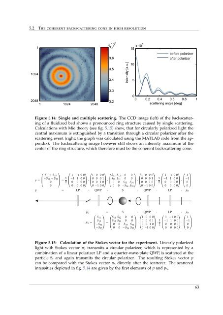
5.2 The coherent backscattering cone in high resolution 1 3.7 3.6 x 10 4 0 0.2 0.4 0.6 0.8 1 15 x 107 scattering angle [deg] before polarizer after polarizer 1024 3.5 3.4 intensity [a.u.] 10 5 3.3 2048 3.2 1 1024 2048 0 Figure 5.14: Single and multiple scattering. The CCD image (left) of the backscattering of a fluidized bed shows a pronounced ring structure caused by single scattering. Calculations with Mie theory (see fig. 5.15) show, that for circularly polarized light the central maximum is extinguished by a transition through a circular polarizer after the scattering event (right; the graph was calculated using the MATLAB code from the appendix). The backscattering image however still shows an intensity maximum at the center of the ring structure, which therefore must be the coherent backscattering cone. ⎛ ⎞ ⎛ ⎞ ⎛ ⎞ ⎛ ⎞ ⎛ ⎞ ⎛ ⎞ ⎛ ⎞ S 11 + S 33 1 −1 0 0 1 0 0 0 S 11 S 12 0 0 1 0 0 0 1 −1 0 0 1 p = ⎜−S 11 − S 33 ⎟ ⎝ 0 ⎠ = 1 ⎜−1 1 0 0 ⎟ 2 ⎝ 0 0 0 0⎠ · ⎜0 0 0 1 ⎟ ⎝0 0 1 0⎠ · ⎜S 12 S 11 0 0 ⎟ ⎝ 0 0 S 33 S 34 ⎠ · ⎜0 0 0 1 ⎟ ⎝0 0 1 0⎠ · 1 ⎜−1 1 0 0 ⎟ 2 ⎝ 0 0 0 0⎠ · ⎜−1 ⎟ ⎝ 0 ⎠ 0 0 0 0 0 0 −1 0 0 0 0 −S 34 S 33 0 −1 0 0 0 0 0 0 0 p = LP · QWP · S · QWP · LP · p 0 p S = S · QWP · LP · p 0 ⎛ ⎞ ⎛ ⎞ ⎛ ⎞ ⎛ ⎞ ⎛ ⎞ S 11 S 11 S 12 0 0 1 0 0 0 1 −1 0 0 1 p S = ⎜ S 12 ⎟ ⎝−S 34 ⎠ = ⎜S 12 S 11 0 0 ⎟ ⎝ 0 0 S 33 S 34 ⎠ · ⎜0 0 0 1 ⎟ ⎝0 0 1 0⎠ · 1 ⎜−1 1 0 0 ⎟ 2 ⎝ 0 0 0 0⎠ · ⎜−1 ⎟ ⎝ 0 ⎠ −S 33 0 0 −S 34 S 33 0 −1 0 0 0 0 0 0 0 Figure 5.15: Calculation of the Stokes vector for the experiment. Linearly polarized light with Stokes vector p 0 transmits a circular polarizer, which is represented by a combination of a linear polarizer LP and a quarter-wave-plate QWP, is scattered at the particle S, and again transmits the circular polarizer. The resulting Stokes vector p can be compared with the Stokes vector p S directly after the scatterer. The scattered intensities depicted in fig. 5.14 are given by the first elements of p and p S . 63
Page 1 and 2:
Dissertation Coherent Backscatterin
Page 3 and 4:
Ein kurzer Überblick Streuung ist
Page 5 and 6:
Ein kurzer Überblick portweglänge
Page 7 and 8:
Contents Ein kurzer Überblick i Da
Page 9 and 10:
1 Introduction There have been many
Page 11 and 12:
2 Theory In scattering theory, the
Page 13 and 14:
2.2 Single scattering - Mie theory
Page 15 and 16:
2.2 Single scattering - Mie theory
Page 17 and 18:
2.3 Random walk and diffusion scatt
Page 19 and 20: 2.3 Random walk and diffusion of pr
Page 21 and 22: 2.4 The influence of boundaries Fig
Page 23 and 24: 2.5 Photon flux from a surface The
Page 25 and 26: 2.6 On polarization and interferenc
Page 27 and 28: 2.6 On polarization and interferenc
Page 29 and 30: 2.7 The theory of coherent backscat
Page 31 and 32: 2.7 The theory of coherent backscat
Page 33 and 34: 3 Setups 3.1 Laser System The key p
Page 35 and 36: 3.2 Wide Angle Setup 1 .0 0 .8 h e
Page 37 and 38: 3.3 Small Angle Setup 1 0.998 0.996
Page 39 and 40: 3.3 Small Angle Setup Figure 3.6: T
Page 41 and 42: 3.4 Time Of Flight Setup Figure 3.8
Page 43 and 44: 4 Samples 4.1 Sample characterizati
Page 45 and 46: 4.1 Sample characterization techniq
Page 47 and 48: 4.2 The samples sample particle siz
Page 49 and 50: 4.2 The samples Figure 4.5: Fluidiz
Page 51 and 52: 5 Experiments 5.1 Conservation of e
Page 53 and 54: 5.1 Conservation of energy in coher
Page 65 and 66: 5.2 The coherent backscattering con
Page 69: 5.2 The coherent backscattering con
Page 77 and 78: 6 Summary The focus of the work pre
Page 79 and 80: Bibliography [1] http://www.schneid
Page 81 and 82: Bibliography [34] E. Larose, L. Mar
Page 83 and 84: Figures and Tables Figures Backscat
Page 85 and 86: Figures and Tables Tables 4.1 Collo
Page 87 and 88: MATLAB codes Angular intensity dist
Page 89 and 90: Evaluation of the wide angle data E
Page 91 and 92: Evaluation of the wide angle data %
Page 93 and 94: Evaluation of the wide angle data f
Page 95 and 96: Evaluation of the small angle data
Page 97 and 98: Evaluation of the small angle data
Page 99: Evaluation of the small angle data
show all

Coherent Backscattering from Multiple Scattering Systems - KOPS ...

Create successful ePaper yourself

Delete template?

Save as template?