Coherent Backscattering from Multiple Scattering Systems - KOPS ...

2 Theory
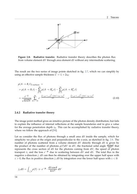
Figure 2.8: Radiative transfer. Radiative transfer theory describes the photon flux
from volume element dV through area element dS without any intermediate scattering.
The result are the two series of image points sketched in fig. 2.7, which we can simplify by
using an effective sample thickness L ′ = L + 2z 0 :
ρ(A → B, t) 2 surfaces =
∞
∑
= ρ(A → B, t) − ρ(A → B ′ ∞
k , t) − ∑
k=1 k=1
ρ(A → B ′′
k , t)
= e− τ
t ∞
√ 3 ∑ e ( − ⃗r ⊥,B −⃗r ⊥,A) 2 +(2mL ′ +z B −z A ) 2
4Dt − e ( − ⃗r ⊥,B −⃗r ⊥,A) 2 +(2mL ′ −z B −z A ) 2
4Dt (2.10)
4πDt m=−∞
2.4.2 Radiative transfer theory
The image point method gives an intuitive picture of the photon density distribution, but fails
to explain the influence of internal reflections at the sample boundaries and to give a value
for the average penetration depth z 0 . This can be accomplished by radiative transfer theory,
where we follow the approach of [58].
Let us consider the flux of photons through a small area dS inside the sample, which for
simplicity we place at the origin and perpendicular to the z-axis, as sketched in fig. 2.8. The
number of photons scattered from a volume element dV directly through dS is given by
dS cos θ
the product of the number of photons ρ(⃗r)dV in dV, the fractional solid angle that
represents the cross section of dS for the photons coming from dV, the speed of photon
transport v, and the loss e − r
l ∗ due to scattering between dV and dS. The total flux in the
negative z-direction j − dS can then be obtained by integrating over the upper half space with
z > 0, the flux in positive direction j + dS by integration over the lower half space with z < 0:
4πr 2
∫
j ∓ dS =
z > < 0 ρ(⃗r) · v · e − r
l ∗ ·
dS cos θ
4πr 2
dV
14