Targets IMage Energy Regional (TIMER) Model, Technical ...

RIVM report 461502024 page 157 of 188
share product 1
0.6
0.5
0.4
0.3
0.2
0.1
ADJT=1
ADJT=5
ADJT=10
ADJT=20
0
0 0.2 0.4 0.6 0.8 1
cross-price elasticity
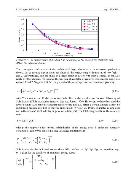
)LJXUH7KHPDUNHWVKDUHRISURGXFWDVIXQFWLRQRIλWKHFURVVSULFHHODVWLFLW\DQG
$'-7WKHDGMXVWPHQWWLPH
The conceptual background of the multinomial logit allocation is in economic production
theory. Let us assume that an actor can chose for his energy supply from a set of two fuels, 1
and 2. Alternatively, one can think of a large group of actors with such a choice. It can also
relate to other choices, for instance the fraction of available or required investments going into
options 1 and 2. Suppose that the energy part of the actor’s production function is given by:
−
β β
[ ] β − −1
D(
) − ) ) + E(
) −
/
< = )
(9.13)
1 10
2 20
)
with Y the output and F I the respective fuels. This is the well-known Constant Elasticity of
Substitution (CES) production function (see e.g. Jones, 1976). However, we have included the
lower bounds F i0 to take into account that for every fuel c.q. option a certain amount cannot be
substituted because it is tied to specific applications (Vries HWDO 1981). Examples coking coal
use in the iron and steel industry or gasoline in transport. The total energy costs for the actor are
now:
( = S +
$/yr (9.14)
1
)
1
S2)
2
with p i the respective fuel prices. Minimisation of the energy costs E under the boundary
condition of eqn. 9.9 is satisfied, using LaGrange multipliers, if:
S
S
1
2
∂<
/ ∂)
=
∂<
/ ∂)
1
2
=
D ⎛ )
2
− )
⎜
E ⎝ )
1
− )
20
10
⎞
⎟
⎠
1+β
(9.15)
Substituting for the indicated market share IMS 2 , defined as F 2 /( F 1 + F 2 ), and rewriting eqn.
9.11 gives for the condition of minimum energy costs:
⎛ ,062
⎞
1/(1+
β ) ⎜ ( ))
1
− )
20 ⎟
⎛ ES1
⎞ ⎜ 1−
,062
=
⎟
⎜
⎟
(9.16)
⎜
⎝ DS
− ⎟
2 ⎠
)
1
)
10
⎜
⎟
⎝
⎠