Dissertation - HQ

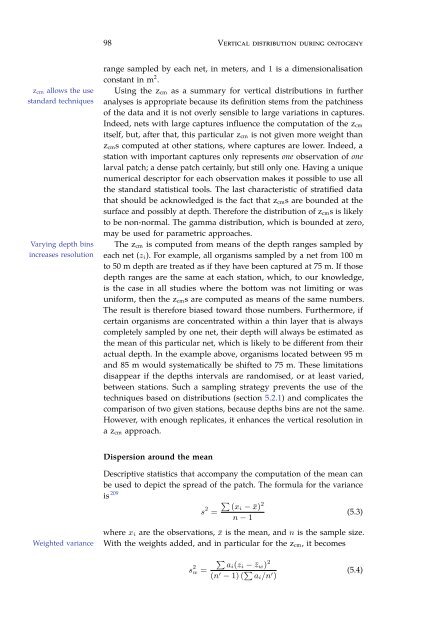
98 Vertical distribution during ontogeny
z cm allows the use
standard techniques
Varying depth bins
increases resolution
range sampled by each net, in meters, and 1 is a dimensionalisation
constant in m 2 .
Using the z cm as a summary for vertical distributions in further
analyses is appropriate because its definition stems from the patchiness
of the data and it is not overly sensible to large variations in captures.
Indeed, nets with large captures influence the computation of the z cm
itself, but, after that, this particular z cm is not given more weight than
z cms computed at other stations, where captures are lower. Indeed, a
station with important captures only represents one observation of one
larval patch; a dense patch certainly, but still only one. Having a unique
numerical descriptor for each observation makes it possible to use all
the standard statistical tools. The last characteristic of stratified data
that should be acknowledged is the fact that z cms are bounded at the
surface and possibly at depth. Therefore the distribution of z cms is likely
to be non-normal. The gamma distribution, which is bounded at zero,
may be used for parametric approaches.
The z cm is computed from means of the depth ranges sampled by
each net (z i). For example, all organisms sampled by a net from 100 m
to 50 m depth are treated as if they have been captured at 75 m. If those
depth ranges are the same at each station, which, to our knowledge,
is the case in all studies where the bottom was not limiting or was
uniform, then the z cms are computed as means of the same numbers.
The result is therefore biased toward those numbers. Furthermore, if
certain organisms are concentrated within a thin layer that is always
completely sampled by one net, their depth will always be estimated as
the mean of this particular net, which is likely to be different from their
actual depth. In the example above, organisms located between 95 m
and 85 m would systematically be shifted to 75 m. These limitations
disappear if the depths intervals are randomised, or at least varied,
between stations. Such a sampling strategy prevents the use of the
techniques based on distributions (section 5.2.1) and complicates the
comparison of two given stations, because depths bins are not the same.
However, with enough replicates, it enhances the vertical resolution in
a z cm approach.
Dispersion around the mean
Weighted variance
Descriptive statistics that accompany the computation of the mean can
be used to depict the spread of the patch. The formula for the variance
is 209 P
s 2 (xi − ¯x) 2
=
(5.3)
n − 1
where x i are the observations, ¯x is the mean, and n is the sample size.
With the weights added, and in particular for the z cm, it becomes
P ai(z
s 2 i − ¯z w) 2
w =
(n ′ − 1) ( P a i/n ′ )
(5.4)