Dissertation - HQ

142 Oceanography vs. behaviour
Simple Euler-forward
advection is appropriate
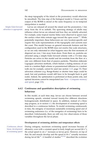
the steep topography of the island or the promontory would otherwise
be smoothed). The time step of the biological model is 3 hours and the
output of the ROMS is stored at the same frequency so no temporal
interpolation is needed.
Larvae are released all around the island and the promontory, 1 km
away from the 10 m isobath. The spawning strategy of adults may
influence where larvae are released and how they are initially advected.
For example, some tropical marine fishes were observed to spawn near
the surface when tides entrain eggs toward the open ocean 185 . While
potentially important, these behaviours are very location-specific and
require fine scale representations of the topography and currents near
the coast. This model focuses on general mesoscale features and the
configuration used in the ROMS does not resolve fine scale structures,
so we are only interested in what happens once the first moments of
dispersal are over, 1 km away from shore. From there on, particles are
advected using a simple Euler forward scheme with a 3 h time step.
Particles are active in this model and de-correlate from the flow at a
rate very different from that of passive particles. Therefore elaborate
Lagragian advection methods, which feature a fading memory of currents
in a random flight scheme or parameterised diffusion in a random
walk one for example, cannot be used (see section 1.4.5, page 35). Finer
advection schemes (e.g. Runge-Kutta) or shorter time steps could be
used, but end positions would still have to be brought back to grid
nodes. Indeed, the optimisation is performed at those points only, and
optimal decisions cannot be interpolated (see Note – Computer memory
and speed, page 129).
6.4.2 Continuous and quantitative description of swimming
behaviour
In this model, at each time step, larvae can choose between several
swimming speeds, oriented toward twenty-five different directions
homogeneously distributed in space. In addition, instead of a three
step progress, as in section 6.3, the development of swimming speed is
described in a continuous fashion. To model swimming continuously
in time, the ontogeny of maximum sustainable swimming speed and of
swimming endurance (i.e. of the energetics of swimming) have to be
described. Unfortunately, there are still very few observations of those
variables throughout the larval phase.
Development of swimming abilities and temperature effects
Continuous, almost
linear, development
of swimming speed
During ontogeny, maximum swimming speed increases because of
allometry: even with a constant speed in body length per second (bl s -1 ),
the actual speed in cm s -1 increases as larvae grow. However, on top of
that, fin and muscle develop and the speed in bl s -1 actually increases
during larval life 95 . A handful of studies 56,57,60 described the evolution