Dissertation - HQ

More documents

Recommendations

Info

120 Oceanography vs. behaviour and time, giving either a real number (current speed) or a probability (to survive or to eat) at each time step. In this simple model, predation pressure, food availability and currents are uniform on the whole space. Survival probability equals the constant p. Food is considered sufficient and the probability to eat is one. Currents are taking the larva away from the coast by a quantity ∆x 0 > 0 at each time step. Controlled dynamics Foraging or swimming At each time step, the larva must resolve a trade-off between two types of behaviour: foraging (decision d = 0) or directional swimming (decision d = 1) a . Each behaviour has consequences on its future state, as described below and in Figure 6.1. Foraging Either the larva dies, or it survives with probability p, increases its energy by a fixed quantity ∆θ 0 , and is taken away by the current on a distance ∆x 0 . 8 < (0, x t) → 1-p (θ t+1, x t+1) = “ : S θmax 0 (θ t + ∆θ 0 )), S xmax ” 0 (x t + ∆x 0 ) → p where “→” means “with probability” and indices denote a function of time (i.e. θ t = θ(t) and x t = x(t)). The S function (saturation) ensures that position and energy stay bounded, and is defined by 8 ξ max S ξ min (ξ) = >< ξ >: ξ max ξ min if ξ > ξ max if ξ ∈ [ξ min, ξ max] if ξ < ξ min Directional swimming Either the larva dies, or it survives with probability p, swims toward the coast, against the current, and travels a distance ∆x 1 . It consumes ∆θ 1 units of energy doing so. 8 < (0, x t) → 1-p (θ t+1, x t+1) = “ : S θmax 0 (θ t − ∆θ 1 )), S xmax ” 0 (x t − ∆x 1 ) → p A controlled Markov chain . . . These probabilities are used to build the transition matrices which characterise the Markov chain (Figure 6.2). An element M(i, j) of such matrices is the probability of transition between the initial state i and the final state j. As the Markov chain is controlled, a different transition matrix is associated with each decision (i.e. control) of the larva. The simplest meaningful transition matrices for this model are presented in Figure 6.2. State is defined by three energy levels and four a In stochastic optimal control, controls (i.e. decisions) are commonly noted using the letter u. To avoid confusion with the zonal (West-East) component of current in a three dimensional flow, which is the u component of a (u, v, w) vector field, decisions are noted d here.
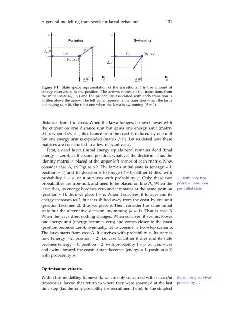
A general modelling framework for larval behaviour 121 Figure 6.1 State space representation of the transitions. θ is the amount of energy reserves, x is the position. The arrows represent the transitions from the initial state (θ t, x t) and the probability associated with each transition is written above the arrow. The left panel represents the transition when the larva is foraging (d = 0), the right one when the larva is swimming (d = 1) distances from the coast. When the larva forages, it moves away with the current on one distance unit but gains one energy unit (matrix M 0 ); when it swims, its distance from the coast is reduced by one unit but one energy unit is expended (matrix M 1 ). Let us detail how these matrices are constructed in a few relevant cases. First, a dead larva (initial energy equals zero) remains dead (final energy is zero), at the same position, whatever the decision. Thus the identity matrix is placed at the upper left corner of each matrix. Now, consider case A, in Figure 6.2. The larva’s initial state is (energy = 1, position = 1) and its decision is to forage (d = 0). Either it dies, with probability 1 − p, or it survives with probability p. Only these two probabilities are non-null, and need to be placed on line A. When the larva dies, its energy becomes zero and it remains at the same position (position = 1); thus we place 1 − p. When it survives, it forages and its energy increases to 2, but it is shifted away from the coast by one unit (position becomes 2); thus we place p. Then, consider the same initial state but the alternative decision: swimming (d = 1). That is case B. When the larva dies, nothing changes. When survives, it swims, looses one energy unit (energy becomes zero) and comes closer to the coast (position becomes zero). Eventually, let us consider a two-step scenario. The larva starts from case A. It survives with probability p. Its state is now (energy = 2, position = 2), i.e. case C. Either it dies and its state becomes (energy = 0, position = 2) with probability 1 − p; or it survives and swims toward the coast: it state becomes (energy = 1, position = 1) with probability p. . . . with only two possible transitions per initial state Optimisation criteria Within this modelling framework, we are only concerned with successful trajectories: larvae that return to where they were spawned at the last time step (i.e. the only possibility for recruitment here). In the simplest Maximising survival probability . . .
Page 3:
À mon étoile.
Page 6 and 7:
vi Résumé La plupart des organism
Page 8 and 9:
viii Abstract Most demersal marine
Page 10 and 11:
x Table des matières 1.3.3 Simple
Page 12 and 13:
xii Table des matières 6.2.3 Examp
Page 14 and 15:
xiv Liste des figures 4.6 Distribut
Page 17:
Liste des tableaux 1.1 Potential or
Page 20 and 21:
2 Introduction La survie des larves
Page 22 and 23:
4 Introduction Limitation par le re
Page 24 and 25:
6 Introduction Les courants déterm
Page 26 and 27:
8 Introduction où m est le taux de
Page 28 and 29:
10 Introduction biologique simple.
Page 30 and 31:
12 Introduction Le milieu lui-même
Page 32 and 33:
14 Introduction Figure I.6 Schémat
Page 34 and 35:
16 Introduction obstacles technique
Page 36 and 37:
18 Introduction Figure I.8 Prédict
Page 38 and 39:
20 Introduction I.5 La biologie des
Page 40 and 41:
22 Introduction du fonctionnement d
Page 42 and 43:
24 Introduction L’objectif de cet
Page 44 and 45:
26 Behaviour in models 1.1 Introduc
Page 46 and 47:
28 Behaviour in models Using mean p
Page 48 and 49:
30 Behaviour in models 1.3 Vertical
Page 50 and 51:
32 Behaviour in models . . . bring
Page 52 and 53:
34 Behaviour in models of measured
Page 54 and 55:
36 Behaviour in models Additive dis
Page 56 and 57:
38 Behaviour in models In situ stud
Page 58 and 59:
40 Behaviour in models Operational
Page 60 and 61:
42 Behaviour in models Effects on p
Page 62 and 63:
44 Behaviour in models begins is no
Page 64 and 65:
46 Behaviour in models 1.10 Conclus
Page 66 and 67:
48 Larvae orientation in situ Diver
Page 68 and 69:
50 Larvae orientation in situ . . .
Page 70 and 71:
52 Larvae orientation in situ optio
Page 72 and 73:
54 Larvae orientation in situ if >
Page 74 and 75:
56 Larvae orientation in situ Table
Page 76 and 77:
58 Larvae orientation in situ that
Page 78 and 79:
60 Larvae orientation in situ 2.A A
Page 80 and 81:
62 Behaviour of settling fishes at
Page 82 and 83:
Page 84 and 85:
Page 87 and 88: Chapter 4 Biophysical correlates in
Page 89 and 90: Methods 71 4.2 Methods 4.2.1 Sampli
Page 91 and 92: Methods 73 Three rotations were com
Page 93 and 94: Methods 75 test really focuses on w
Page 95 and 96: Results 77 Figure 4.3 Mean of insta
Page 97 and 98: Results 79 Figure 4.5 Perspective v
Page 99 and 100: Results 81 Table 4.1 Abundances of
Page 101 and 102: Results 83 Figure 4.8 Distribution
Page 103 and 104: Results 85 Figure 4.10 Concentratio
Page 105 and 106: Discussion 87 Figure 4.11 Compariso
Page 107 and 108: Discussion 89 But the most likely e
Page 109 and 110: Acknowledgements 91 This evidence a
Page 111 and 112: Chapter 5 Ontogenetic vertical “m
Page 113 and 114: The statistical analysis of vertica
Page 119 and 120: Methods 101 80, 55, 30 m (Figure 4.
Page 121 and 122: Methods 103 same station were likel
Page 123 and 124: Results 105 Figure 5.2 Univariate r
Page 125 and 126: Results 107 5.4.3 Ontogenetic shift
Page 127 and 128: Results 109 Figure 5.5 Violin plot
Page 129 and 130: Discussion 111 5.5 Discussion 5.5.1
Page 131 and 132: Discussion 113 expression of differ
Page 133 and 134: Chapter 6 Oceanography vs. behaviou
Page 135 and 136: Introduction 117 a good description
Page 137: A general modelling framework for l
Page 141 and 142: A general modelling framework for l
Page 143 and 144: A general modelling framework for l
Page 145 and 146: The balance between feeding and pre
Page 155 and 156: Oriented swimming and passive advec
Page 179 and 180: General discussion 161 such integra
Page 181 and 182: General discussion 163 6.5.2 Why se
Page 183 and 184: General discussion 165 such as the
Page 185 and 186: General discussion 167 energeticall
Page 187: Acknowledgements 169 Therefore: •
Page 190 and 191:
172 Conclusion Un environnement pé
Page 192 and 193:
174 Conclusion global sur la connec
Page 194 and 195:
176 Conclusion l’intérêt est po
Page 196 and 197:
178 Conclusion La différence entre
Page 198 and 199:
180 Conclusion Mieux décrire la di
Page 200 and 201:
182 Conclusion Comme tout comportem
Page 202 and 203:
184 Undescribed Chaetodonthidae Fig
Page 204 and 205:
186 Undescribed Chaetodonthidae Fig
Page 206 and 207:
188 Bibliographie [12] Cushing DH.
Page 208 and 209:
190 Bibliographie [39] Johnson MW.
Page 210 and 211:
192 Bibliographie [71] Paris CB, Co
Page 212 and 213:
194 Bibliographie [99] Lara MR. Mor
Page 214 and 215:
196 Bibliographie [127] Masuda R, S
Page 216 and 217:
198 Bibliographie [157] Holbrook SJ
Page 218 and 219:
200 Bibliographie [187] Bowen B, Ba
Page 220 and 221:
202 Bibliographie [218] Oxenford HA
Page 222 and 223:
204 Bibliographie [246] Wellington
Page 224 and 225:
206 Bibliographie [276] Sargent RC,
Page 226 and 227:
208 Bibliographie [308] Greenberg D
Page 228 and 229:
210 Remerciements solides pour ces
Page 230 and 231:
212 Remerciements tri des larves de
Page 232:
214 Remerciements Évidemment, tout
show all

Dissertation - HQ

You also want an ePaper? Increase the reach of your titles

Delete template?

Save as template?