- Page 2 and 3:
Authors: Dr. rer. nat. Jochen Broz
- Page 4 and 5:
2 Part 3. Reference Manual 3.1 Netl
- Page 7 and 8:
A Short Introduction 1.1 Welcome to
- Page 9 and 10:
1.1 Welcome to Analog Insydes 7 Net
- Page 11 and 12:
1.2 Getting Started 9 (Section 3.6.
- Page 13 and 14:
1.2 Getting Started 11 CancelTerms
- Page 15 and 16:
1.2 Getting Started 13 Analysis Tas
- Page 17 and 18:
1.2 Getting Started 15 this topic i
- Page 19 and 20:
1.2 Getting Started 17 In[10]:= ref
- Page 21 and 22:
1.2 Getting Started 19 In[16]:= op7
- Page 23 and 24:
1.2 Getting Started 21 The numerica
- Page 25 and 26:
1.2 Getting Started 23 comparison o
- Page 27 and 28:
1.3 What’s New 25 1.3 What’s Ne
- Page 29 and 30:
1.3 What’s New 27 Graphics Functi
- Page 31 and 32:
1.3 What’s New 29 Modeling Langua
- Page 33:
1.3 What’s New 31 NDAESolve, NDAE
- Page 36 and 37:
34 2. Tutorial 2.1 Preface 2.1.1 Ho
- Page 38 and 39:
36 2. Tutorial The Netlist command
- Page 40 and 41:
38 2. Tutorial {V0, {1, 2}, V0} Hen
- Page 42 and 43:
40 2. Tutorial Controlled Sources:
- Page 44 and 45:
42 2. Tutorial In[9]:= vdeqs = Circ
- Page 46 and 47:
44 2. Tutorial the Symbolic option
- Page 48 and 49:
46 2. Tutorial In[16]:= cccseqs2 =
- Page 50 and 51:
48 2. Tutorial 2.3 Circuits and Sub
- Page 52 and 53:
50 2. Tutorial Model[ Name −> sub
- Page 54 and 55:
52 2. Tutorial Connections to subci
- Page 56 and 57:
54 2. Tutorial In[2]:= commonEmitte
- Page 58 and 59:
56 2. Tutorial In[5]:= flatAmpDyn =
- Page 60 and 61:
58 2. Tutorial 2.3.5 Subcircuit Par
- Page 62 and 63:
60 2. Tutorial In[13]:= darlington
- Page 64 and 65:
62 2. Tutorial same global symbols
- Page 66 and 67:
64 2. Tutorial appropriate Scope ar
- Page 68 and 69:
66 2. Tutorial B C E RB gm*VBE E Fi
- Page 70 and 71:
68 2. Tutorial In[27]:= Circuit[ Mo
- Page 72 and 73:
70 2. Tutorial An advanced applicat
- Page 74 and 75:
72 2. Tutorial 2.4 Setting up and S
- Page 76 and 77:
74 2. Tutorial To illustrate equati
- Page 78 and 79:
76 2. Tutorial 2.4.3 Circuit Equati
- Page 80 and 81:
78 2. Tutorial In[10]:= CircuitEqua
- Page 82 and 83:
80 2. Tutorial 2.4.4 Additional Opt
- Page 84 and 85:
82 2. Tutorial In[18]:= rlc2eqs = C
- Page 86 and 87:
84 2. Tutorial In[3]:= BodePlot[H1[
- Page 88 and 89:
86 2. Tutorial In[6]:= H12a[s_] :=
- Page 90 and 91:
88 2. Tutorial In[11]:= NicholPlot[
- Page 92 and 93:
90 2. Tutorial In[14]:= RootLocusPl
- Page 94 and 95:
92 2. Tutorial 2.6 Modeling and Ana
- Page 96 and 97:
94 2. Tutorial Model[ Name −> Dio
- Page 98 and 99:
96 2. Tutorial 2.6.3 Referencing Be
- Page 100 and 101:
98 2. Tutorial In[8]:= dnwsol = Com
- Page 102 and 103:
100 2. Tutorial the base current, i
- Page 104 and 105:
102 2. Tutorial Similarly, we defin
- Page 106 and 107:
104 2. Tutorial In[14]:= mnaeqsfa =
- Page 108 and 109:
106 2. Tutorial 2.7 Time-Domain Ana
- Page 110 and 111:
108 2. Tutorial Let’s use NDAESol
- Page 112 and 113:
110 2. Tutorial The influence of th
- Page 114 and 115:
112 2. Tutorial In[11]:= diffAmp =
- Page 116 and 117:
114 2. Tutorial Additionally, we fo
- Page 118 and 119:
116 2. Tutorial Then, we run NDAESo
- Page 120 and 121:
118 2. Tutorial 2.7.3 Flow of Trans
- Page 122 and 123:
120 2. Tutorial input of circuit ne
- Page 124 and 125: 122 2. Tutorial difference between
- Page 126 and 127: 124 2. Tutorial Vic 1 2 L1 C1 R1 Io
- Page 128 and 129: 126 2. Tutorial In[30]:= oscillator
- Page 130 and 131: 128 2. Tutorial In[36]:= TransientP
- Page 132 and 133: 130 2. Tutorial 2.8 Linear Symbolic
- Page 134 and 135: 132 2. Tutorial Even for this very
- Page 136 and 137: 134 2. Tutorial than R3 and R4: R1
- Page 138 and 139: 136 2. Tutorial Let’s apply solut
- Page 140 and 141: 138 2. Tutorial at all. This will b
- Page 142 and 143: 140 2. Tutorial s ⩵ Π I f . Fi
- Page 144 and 145: 142 2. Tutorial In[33]:= voutsimp3
- Page 146 and 147: 144 2. Tutorial of all terms by lea
- Page 148 and 149: 146 2. Tutorial D G S VGS gm*VGS GD
- Page 150 and 151: 148 2. Tutorial 6 VDD M3 M4 5 1 M1
- Page 152 and 153: 150 2. Tutorial Ys ⩵ Hs Xs Hence
- Page 154 and 155: 152 2. Tutorial 2.9.3 Device Mismat
- Page 156 and 157: 154 2. Tutorial In[17]:= cmgSAG = A
- Page 158 and 159: 156 2. Tutorial Replacing the load
- Page 160 and 161: 158 2. Tutorial Stimulus Sources fo
- Page 162 and 163: 160 2. Tutorial In[27]:= twoportmna
- Page 164 and 165: 162 2. Tutorial Let’s examine the
- Page 166 and 167: 164 2. Tutorial In[45]:= BodePlot[r
- Page 168 and 169: 166 2. Tutorial Finally, we verify
- Page 170 and 171: 168 2. Tutorial each input symbol (
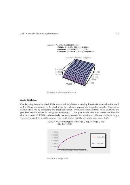
- Page 172 and 173: 170 2. Tutorial As a first step we
- Page 176 and 177: 174 2. Tutorial In[16]:= Max @ Map[
- Page 178 and 179: 176 2. Tutorial In[24]:= Statistics
- Page 180 and 181: 178 2. Tutorial the equations for t
- Page 182 and 183: 180 3. Reference Manual 3.1 Netlist
- Page 184 and 185: 182 3. Reference Manual A complex c
- Page 186 and 187: 184 3. Reference Manual This netlis
- Page 188 and 189: 186 3. Reference Manual You may not
- Page 190 and 191: 188 3. Reference Manual If no value
- Page 192 and 193: 190 3. Reference Manual A model ref
- Page 194 and 195: 192 3. Reference Manual 3.2 Subcirc
- Page 196 and 197: 194 3. Reference Manual Name −> "
- Page 198 and 199: 196 3. Reference Manual Ports Ports
- Page 200 and 201: 198 3. Reference Manual Any symbol
- Page 202 and 203: 200 3. Reference Manual calculated
- Page 204 and 205: 202 3. Reference Manual Definition
- Page 206 and 207: 204 3. Reference Manual (ODEs). In
- Page 208 and 209: 206 3. Reference Manual With the In
- Page 210 and 211: 208 3. Reference Manual A circuit w
- Page 212 and 213: 210 3. Reference Manual This code d
- Page 214 and 215: 212 3. Reference Manual Simulate th
- Page 216 and 217: 214 3. Reference Manual option name
- Page 218 and 219: 216 3. Reference Manual 3.3.3 FindM
- Page 220 and 221: 218 3. Reference Manual 3.3.6 LoadM
- Page 222 and 223: 220 3. Reference Manual option name
- Page 224 and 225:
222 3. Reference Manual Remove the
- Page 226 and 227:
224 3. Reference Manual option name
- Page 228 and 229:
226 3. Reference Manual When HoldMo
- Page 230 and 231:
228 3. Reference Manual List the Mo
- Page 232 and 233:
230 3. Reference Manual option name
- Page 234 and 235:
232 3. Reference Manual option name
- Page 236 and 237:
234 3. Reference Manual Controlling
- Page 238 and 239:
236 3. Reference Manual Value Symbo
- Page 240 and 241:
238 3. Reference Manual If the Inde
- Page 242 and 243:
240 3. Reference Manual Value takes
- Page 244 and 245:
242 3. Reference Manual Set up a sy
- Page 246 and 247:
244 3. Reference Manual Set up a sy
- Page 248 and 249:
246 3. Reference Manual Now we use
- Page 250 and 251:
248 3. Reference Manual Replace all
- Page 252 and 253:
250 3. Reference Manual 3.5.2 ACEqu
- Page 254 and 255:
252 3. Reference Manual Show equati
- Page 256 and 257:
254 3. Reference Manual Define netl
- Page 258 and 259:
256 3. Reference Manual Extract val
- Page 260 and 261:
258 3. Reference Manual 3.6.1 AddEl
- Page 262 and 263:
260 3. Reference Manual Examples Lo
- Page 264 and 265:
262 3. Reference Manual Display net
- Page 266 and 267:
264 3. Reference Manual Define a si
- Page 268 and 269:
266 3. Reference Manual 3.6.9 GetPa
- Page 270 and 271:
268 3. Reference Manual Return the
- Page 272 and 273:
270 3. Reference Manual You can set
- Page 274 and 275:
272 3. Reference Manual the DesignP
- Page 276 and 277:
274 3. Reference Manual Show new DA
- Page 278 and 279:
276 3. Reference Manual Show update
- Page 280 and 281:
278 3. Reference Manual Match symbo
- Page 282 and 283:
280 3. Reference Manual number of e
- Page 284 and 285:
282 3. Reference Manual 3.7 Numeric
- Page 286 and 287:
284 3. Reference Manual The combina
- Page 288 and 289:
286 3. Reference Manual The default
- Page 290 and 291:
288 3. Reference Manual have to be
- Page 292 and 293:
290 3. Reference Manual Read the ne
- Page 294 and 295:
292 3. Reference Manual 3.7.5 NDAES
- Page 296 and 297:
294 3. Reference Manual option name
- Page 298 and 299:
296 3. Reference Manual Note that t
- Page 300 and 301:
298 3. Reference Manual MaxDelta On
- Page 302 and 303:
300 3. Reference Manual In case of
- Page 304 and 305:
302 3. Reference Manual Perform num
- Page 306 and 307:
304 3. Reference Manual Vic 1 2 L1
- Page 308 and 309:
306 3. Reference Manual 3.8 Pole/Ze
- Page 310 and 311:
308 3. Reference Manual r v ⩵
- Page 312 and 313:
310 3. Reference Manual Calculate b
- Page 314 and 315:
312 3. Reference Manual Read in a P
- Page 316 and 317:
314 3. Reference Manual Show the ro
- Page 318 and 319:
316 3. Reference Manual option name
- Page 320 and 321:
318 3. Reference Manual A ϑ i B
- Page 322 and 323:
320 3. Reference Manual Find the po
- Page 324 and 325:
322 3. Reference Manual option name
- Page 326 and 327:
324 3. Reference Manual ErrorFuncti
- Page 328 and 329:
326 3. Reference Manual error but s
- Page 330 and 331:
328 3. Reference Manual If you set
- Page 332 and 333:
330 3. Reference Manual Set up syst
- Page 334 and 335:
332 3. Reference Manual 3.9 Graphic
- Page 336 and 337:
334 3. Reference Manual option name
- Page 338 and 339:
336 3. Reference Manual Automatic s
- Page 340 and 341:
338 3. Reference Manual Display all
- Page 342 and 343:
340 3. Reference Manual Show magnit
- Page 344 and 345:
342 3. Reference Manual Reduce the
- Page 346 and 347:
344 3. Reference Manual 3.9.3 Nicho
- Page 348 and 349:
346 3. Reference Manual Examples Lo
- Page 350 and 351:
348 3. Reference Manual NyquistPlot
- Page 352 and 353:
350 3. Reference Manual Draw a Nyqu
- Page 354 and 355:
352 3. Reference Manual Display the
- Page 356 and 357:
354 3. Reference Manual option name
- Page 358 and 359:
356 3. Reference Manual Examples Lo
- Page 360 and 361:
358 3. Reference Manual Change the
- Page 362 and 363:
360 3. Reference Manual Parametric
- Page 364 and 365:
362 3. Reference Manual Define netl
- Page 366 and 367:
364 3. Reference Manual Generate a
- Page 368 and 369:
366 3. Reference Manual 3.10 Interf
- Page 370 and 371:
368 3. Reference Manual Options Des
- Page 372 and 373:
370 3. Reference Manual Read and co
- Page 374 and 375:
372 3. Reference Manual Independent
- Page 376 and 377:
374 3. Reference Manual Linear resi
- Page 378 and 379:
376 3. Reference Manual ReadNetlist
- Page 380 and 381:
378 3. Reference Manual See also: W
- Page 382 and 383:
380 3. Reference Manual Read simula
- Page 384 and 385:
382 3. Reference Manual DataLabels
- Page 386 and 387:
384 3. Reference Manual option name
- Page 388 and 389:
386 3. Reference Manual Generate th
- Page 390 and 391:
388 3. Reference Manual Define an A
- Page 392 and 393:
390 3. Reference Manual The fourth
- Page 394 and 395:
392 3. Reference Manual Simplify th
- Page 396 and 397:
394 3. Reference Manual option name
- Page 398 and 399:
396 3. Reference Manual be a number
- Page 400 and 401:
398 3. Reference Manual This netlis
- Page 402 and 403:
400 3. Reference Manual Plot the ex
- Page 404 and 405:
402 3. Reference Manual This netlis
- Page 406 and 407:
404 3. Reference Manual The rules m
- Page 408 and 409:
406 3. Reference Manual An example
- Page 410 and 411:
408 3. Reference Manual V and V a
- Page 412 and 413:
410 3. Reference Manual option name
- Page 414 and 415:
412 3. Reference Manual Show compre
- Page 416 and 417:
414 3. Reference Manual Clusterboun
- Page 418 and 419:
416 3. Reference Manual Examples Lo
- Page 420 and 421:
418 3. Reference Manual As mentione
- Page 422 and 423:
420 3. Reference Manual 3.13 Miscel
- Page 424 and 425:
422 3. Reference Manual The main pu
- Page 426 and 427:
424 3. Reference Manual ThicknessFu
- Page 428 and 429:
426 3. Reference Manual 3.13.3 Math
- Page 430 and 431:
428 3. Reference Manual View global
- Page 432 and 433:
430 3. Reference Manual Use full-pr
- Page 434 and 435:
432 3. Reference Manual wish to run
- Page 436 and 437:
434 3. Reference Manual 3.15 The An
- Page 438 and 439:
436 3. Reference Manual 3.15.3 Rele
- Page 441 and 442:
Appendix 4.1 Stimuli Sources . . .
- Page 443 and 444:
4.1 Stimuli Sources 441 argument na
- Page 445 and 446:
4.1 Stimuli Sources 443 4.1.3 Pulse
- Page 447 and 448:
4.1 Stimuli Sources 445 Examples Lo
- Page 449 and 450:
4.1 Stimuli Sources 447 A CheckedSi
- Page 451 and 452:
4.2 Netlist Elements 449 element ty
- Page 453 and 454:
4.2 Netlist Elements 451 Modified n
- Page 455 and 456:
4.2 Netlist Elements 453 4.2.9 Curr
- Page 457 and 458:
4.2 Netlist Elements 455 node−, r
- Page 459 and 460:
4.2 Netlist Elements 457 For infini
- Page 461 and 462:
4.2 Netlist Elements 459 4.2.20 Sig
- Page 463 and 464:
4.2 Netlist Elements 461 input T ou
- Page 465 and 466:
4.3 Model Library 463 Anode: Cathod
- Page 467 and 468:
4.3 Model Library 465 parameter nam
- Page 469 and 470:
4.3 Model Library 467 Small-Signal
- Page 471 and 472:
4.3 Model Library 469 Base: Collect
- Page 473 and 474:
4.3 Model Library 471 parameter nam
- Page 475 and 476:
4.3 Model Library 473 parameter nam
- Page 477 and 478:
4.3 Model Library 475 parameter nam
- Page 479 and 480:
4.3 Model Library 477 parameter nam
- Page 481 and 482:
4.3 Model Library 479 parameter nam
- Page 483 and 484:
4.3 Model Library 481 D CGB RD CGD
- Page 485 and 486:
4.3 Model Library 483 parameter nam
- Page 487 and 488:
4.3 Model Library 485 parameter nam
- Page 489 and 490:
4.3 Model Library 487 Small-Signal
- Page 491 and 492:
4.3 Model Library 489 s*Cdd*vd s*Cd
- Page 493 and 494:
4.3 Model Library 491 parameter nam
- Page 495 and 496:
4.3 Model Library 493 parameter nam
- Page 497 and 498:
4.3 Model Library 495 D RD igd CGD
- Page 499 and 500:
4.3 Model Library 497 parameter nam
- Page 501 and 502:
4.3 Model Library 499 parameter nam
- Page 503 and 504:
Index ABM (analog behavioral model)
- Page 505 and 506:
Index Design points — GetDesignPo
- Page 507 and 508:
Index Junction field-effect transis
- Page 509 and 510:
Index OperatingPointPostfix — Rea
- Page 511 and 512:
Index SinWave — Transistor models