Contents Telektronikk - Telenor

While enforcing the PCR, the resulting
picture quality was assessed by a small
group of people in terms of flicker, loss
of picture, etc. We discovered that besides
the value of the cell loss ratio, also
the structure of the cell loss process (e.g.
correlated cell losses) has a strong influence
on the picture quality. However, the
current definition of network performance
in (5) does not include parameters
to describe this structure of the cell loss
process.
3 Experiments on Connection
Admission Control
The aim of the CAC experiments is to
investigate the ability of different CAC
algorithms to maintain network performance
objectives while exploiting the
achievable multiplexing gain as much as
possible. We focus on the Cell Loss
Ratio (CLR) (defined in (5)) as network
performance parameter in our studies.
Our performance study of various CAC
algorithms is not restricted to the twolevel
CAC implementation in the ETB
(see (7) for a description).
In a first step we measure the CLR at a
multiplexer which is fed by several traffic
sources. By varying the number and
the type of the sources we can determine
the admissible number of sources for a
given CLR objective. The set of these
points is referred to as the admission
boundary. Once we have a measured
admission boundary it can be compared
with the corresponding boundaries obtained
when applying a certain CAC
mechanism. If the CAC boundary is
above the measured boundary, the investigated
CAC performs a too optimistic
bandwidth allocation and is not able to
maintain network performance objectives.
On the other hand, if the CAC
boundary is below the measured boundary
the available resources may not be
optimally used by the CAC mechanism.
We have selected CAC algorithms based
on a bufferless model of the multiplexer,
since the small buffers in the ETB
switches can only absorb cell level congestion.
In this paper we only consider
the well-known convolution approach.
Results for other mechanisms can be
found in a more detailed report (10).
Figure 8 depicts the configuration. The
cells generated by N sources are all multiplexed
in the multiplexer under test, but
first the cell streams pass another multiplexing
network where the characteristics
can be modified. It is ensured that cells
are only lost by buffer overflow at the
multiplexer under test. Since the number
of currently available real sources and
applications in the ETB is limited, we
have used ATM test equipment for the
generation of statistical traffic with various
profiles. Multiplexing has been performed
at an output link where a buffer
size of 48 cells and an output capacity of
155.52 Mbit/s are available. The CLR
has been measured for the aggregate traffic.
This is taken into account for the
convolution algorithm by applying the
global information loss criterion (6) for
the calculation of the expected overall
cell loss probability.
3.1 Homogeneous
traffic mix
Source 1
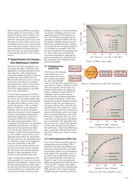
First the case of a homogeneous
traffic mix is considered
where all sources
have identical characteris- Source N
tics. The same ON/OFF
sources as for the UPC experiments have
been used (see Table 1). Figures 9 and 10
show the measured cell loss ratio as a
function of the number of multiplexed
sources. Simulation results with 95 %
confidence intervals and analytical
results from the convolution algorithm
are included in the figures. When comparing
measurement, simulation and convolution
results, the convolution gives
the largest cell loss ratio, while the measurement
shows the smallest loss values.
This is expected, since the convolution is
based on a bufferless model of the multiplexer
such that buffering of cells at the
burst level is neglected. The very good
coincidence of measurement and simulation
is remarkable. The admissible number
of sources for a given CLR objective
can be easily obtained from the figures.
For traffic type 1 almost no multiplexing
gain is achievable while the lower peak
cell rate of traffic type 2 allows a reasonable
gain.
3.2 Heterogeneous traffic mix
Now sources from both traffic types are
multiplexed and the resulting CLR is
measured. The following definition has
been used to determine the set of admission
boundary points: for each boundary
point adding only one further source of
any traffic type would already increase
the resulting CLR above the objective.
Figures 11 and 12 show the measured
admission boundaries for CLR objectives
of 10-4 and 10-6 , together with analytic
results for the convolution algorithm and
PCR allocation. The results reveal that
multiplexing gain can only be achieved
Cell Discard Ratio
Cell Discard Ratio
Cell Discard Ratio
10 0
10 -2
10 -4
10 -6
10 -8
0 10 20 30 40 50
CDV Tolerance τ [cell slots at 622 Mbit/s]
Figure 8 Configuration for the CAC experiments
10 0
10 -2
10 -4
10 -6
10 -8
10 0
10 -2
10 -4
Figure 7 CDR for video traffic
Multiplexing
Network
p=PCR contracted /PCR source
Multiplexer
under test
p=0.940
p=0.986
p=1.003
p=1.074
p=1.157
ATM Traffic
Analyser
Measurement
Simulation
Convolution
4 8 12 16 20
Number of Type 1 Sources
Figure 9 CLR at the multiplexer, type 1
10-6 10-8 Measurement
Simulation
Convolution
110 130 150 170 190
Number of Type 2 Sources
Figure 10 CLR at the multiplexer, type 2
171