Contents Telektronikk - Telenor

214
M
0
0 1
For the sake of simplicity we assume
M ≥ uj ; j = 1,...,P where uj is the workload
from the periodic source and is
given by
uj = max{U(k,j); k = j - 1, j - 2...} (3.20)
(If M < uj for some j one may redefine
the periodic stream by taking
d †
j = dj - (uj - M) if uj > M and
d †
j = dj if uj ≤ M. In this case the workload
from the periodic source may be calculated
by uj = max[min[uj-1 , M] - 1,0]
+ dj . For the redefined system M ≥ u †
j
will be fulfilled, however, one must
count for the extra losses dj - d †
j .)
By examining (3.19) we see that for the
major part of the queue-length distribution
is of the same form as for the infinite
buffer case:
(3.21)
which is valid for i = 0,1,...,M-wk (the
white area in figure 3) where
wk = max{U(k,j); (3.22)
j = k + 1, k + 2, ...
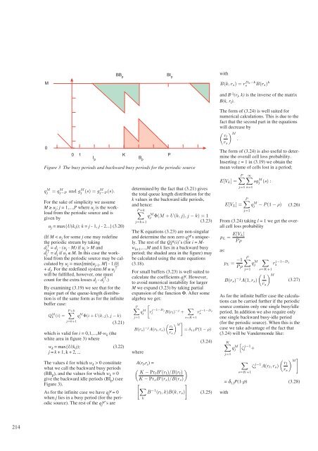
The values k for which wk > 0 constitute
what we call the backward busy periods
(BBp ), and the values for which wk = 0
give the backward idle periods (BIp ) (see
Figure 3).
As for the infinite case we have q M
j = 0
when j lies in a busy period (for the periodic
source). The rest of the q M’s j are
I p
BB p
K P
B p
Figure 3 The busy periods and backward busy periods for the periodic source
q M j = q M j−P and g M j (s) =g M j−P (s).
Q M k (i) =
P �+k
j=k+1
q M j Φ(i + U(k, j),j− k)
determined by the fact that (3.21) gives
the total queue length distribution for the
k values in the backward idle periods,
and hence:
P �+k
q
(3.23)
M j Φ(M + U(k, j),j− k) =1
j=k+1
The K equations (3.23) are non-singular
and determine the non zero q M’s j uniquely.
The rest of the Q M(i)’s k (for i = Mwk+1
,...,M and k lies in a backward busy
period; the shaded area in the figure) may
be calculated using the state equations
(3.18).
For small buffers (3.23) is well suited to
calculate the coefficients qM. j However,
to avoid numerical instability for larger
M we expand (3.23) by taking partial
expansion of the function Φ. After some
algebra we get:
P�
j=1
q M j
where
�
B(rs) −j A(rl,rs)
BI p
A(rl ,rs ) =
�
K − PrlB ′ (rl)/B(rl)
K − PrsB ′ �
(rs)/B(rs)
�
�
B −1 �
(rl,k)B(k, rs)
k
r j−1−Dj
l B(rl) −j + �
� rl
rs
s=K+1
r j−1−Dj
s
� �
M
= δ1,lP (1 − ρ)
(3.24)
(3.25)
with
B(k, rs) =r Dk−k
s B(rs) k
and B -1 (r l , k) is the inverse of the matrix
B(k, r l ).
The form of (3.24) is well suited for
numerical calculations. This is due to the
fact that the second part in the equations
will decrease by
� �M rl
.
The form of (3.24) is also useful to determine
the overall cell loss probability.
Inserting z = 1 in (3.19) we obtain the
mean volume of cells lost in a period;
E[VL] =
(3.26)
From (3.24) taking l = 1 we get the overall
cell loss probability
as:
rs
(3.27)
As for the infinite buffer case the calculations
can be carried further if the periodic
source contains only one single busy/idle
period. In addition we also require only
one single backward busy-idle period
(for the periodic source). When this is the
case we take advantage of the fact that
(3.24) will be Vandermonde like:
with
E[VL] =
pL = E[VL]
Pρ
pL = −1
Pρ
P� ∞�
j=1 s=1
sg M j (s) :
P�
q M j − P (1 − ρ)
j=1
P�
j=1
q M j
�
B(rs) −j �
1
A(1,rs)
K�
j=1
q M j
�
ζ j−1
l
�
s=K+1
+
r
s=K+1
j−1−Dj
s
�M rs
ζ j−1
�
rl
s A(rl,rs)
rs
� M �
= δ 1,l P(1-ρ) (3.28)