

Contents Telektronikk - Telenor
Contents Telektronikk - Telenor
Contents Telektronikk - Telenor

Create successful ePaper yourself
Turn your PDF publications into a flip-book with our unique Google optimized e-Paper software.
34<br />
Since Gw (t) is the survivor function, it<br />
means the probability of the last previous<br />
arrival still being in the system. If the<br />
arrival interval distribution is given by<br />
density f(t), then P{t < arrival interval ≤t<br />
+ dt} = f(t) ⋅ dt. The product of the two<br />
independent terms, G w (t) ⋅ f(t)dt, implies<br />
that the next arrival happens in the interval<br />
(t, t + dt), and that there is still one or<br />
more customers in the system. By integration<br />
over all t we obtain the implicit<br />
equation for determination of σ:<br />
� ∞<br />
σ = e −µ(1−σ)·t · f(t)dt<br />
0<br />
(93)<br />
It is immediately seen that if f(t) = λe –λt ,<br />
then σ = λ/µ, and we get the M/M/1<br />
solution as we should.<br />
By analogy it is clear that the mean values<br />
of waiting and sojourn times, which<br />
are related to calls arriving, and queue<br />
lengths as observed by arriving calls, are<br />
given by formulas identical to those of<br />
M/M/1, only that the mean load A is<br />
replaced by the arrival related load σ.<br />
Taken over time the mean values of number<br />
in queue (Lq ) and number in system<br />
(Ls ) are found by Little’s formula, based<br />
on mean waiting time:<br />
Lq = λ · W =<br />
λ · s · σ<br />
1 − σ<br />
= A · σ<br />
1 − σ<br />
λ · s A<br />
Ls = λ · (W + s) = = (94)<br />
1 − σ 1 − σ<br />
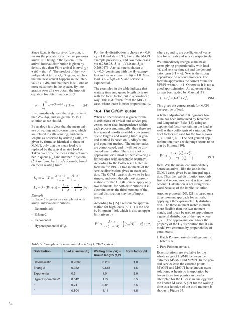
Example<br />
In Table 5 is given an example set with<br />
arrival interval distributions:<br />
- Deterministic<br />
- Erlang-2<br />
- Exponential<br />
- Hyperexponential (H2 ).<br />
Table 5 Example with mean load A = 0.5 of GI/M/1 system<br />
For the H2-distribution is chosen p = 0.9,<br />
λ1 = 1.0 and λ2 = 1/11, like in the M/G/1<br />
example previously, and two more cases:<br />
p = 0.75/0.95, λ1 = 1.0/1.0 and λ2 =<br />
0.2/0.0476. Arrival rate is chosen at<br />
λ = 0.5 (consistent with the H2-examp les) and service time s = 1/µ = 1.0. Mean<br />
load is A = λ/µ = 0.5, and service is<br />
exponential.<br />
The examples in the table indicate that<br />
waiting time and queue length increase<br />
with the form factor, but in a non-linear<br />
way. This is different from the M/G/1<br />
case, where there is strict proportionality.<br />
16.4 The GI/GI/1 queue<br />
When no specification is given for the<br />
distributions of arrival and service processes,<br />
other than independence within<br />
each process and mutually, then there are<br />
few general results available concerning<br />
queue lengths and waiting time. A general<br />
method is based on Lindley’s integral<br />
equation method. The mathematics<br />
are complicated, and it will not be discussed<br />
any further. There are a lot of<br />
approximations, most of them covering a<br />
limited area with acceptable accuracy.<br />
According to the Pollaczek/Khintchine<br />
formula for M/GI/1 two moments of the<br />
service distribution gives an exact solution.<br />
The GI/M1 case is shown to be less<br />
simple, and even though most approximations<br />
for the GI/GI/1 queue apply only<br />
two moments for both distributions, it is<br />
clear that even the third moment of the<br />
arrival distribution may be of importance.<br />
According to [15] a reasonable approximation<br />
for high loads (A→ 1) is the one<br />
by Kingman [16], which is also an upper<br />
limit given by<br />
�<br />
W ≈<br />
(95)<br />
A · s<br />
2 · (1 − A) ·<br />
�<br />
(ca/A) 2 + c 2 s<br />
Distribution Load at arrival (σσ) Waiting time (W) = Form factor (εε)<br />
Queue length (L)/λλ<br />
Deterministic 0.2032 0.255 1.0<br />
Erlang-2 0.382 0.618 1.5<br />
Exponential 0.5 1.0 2.0<br />
Hyperexponential-2 0.642 1.79 3.5<br />
" 0.74 2.85 6.5<br />
" 0.804 4.11 11.5<br />
where ca and cs are coefficient of variation<br />
for arrivals and service respectively.<br />
We immediately recognise the basic<br />
terms giving proportionality with load<br />
(A) and service time (s) and the denominator<br />
term 2(1 – A). Next is the strong<br />
dependence on second moments. The<br />
formula approaches the correct value for<br />
M/M/1 when A → 1. Otherwise it is not a<br />
good approximation. An adjustment factor<br />
has been added by Marchal [17]:<br />
(1 + c 2<br />
s )/(1/A2 + cs2 ) (96)<br />
This gives the correct result for M/G/1<br />
irrespective of load.<br />
A better adjustment to Kingman’s formula<br />
has been introduced by Kraemer<br />
and Langenbach-Belz [18], using an<br />
exponential factor containing the load as<br />
well as the coefficients of variation. Distinct<br />
factors are used for the two regions<br />
ca ≤ 1 and ca ≥ 1. The best general approximation<br />
over a wide range seems to be<br />
that by Kimura [19]:<br />
(97)<br />
Here, σ is the mean load immediately<br />
before an arrival, like the one in the<br />
GI/M/1 case, given by an integral equation.<br />
Thus the real distribution (not only<br />
first and second moments) is taken into<br />
account. Calculation is not straightforward<br />
because of the implicit solution.<br />
Another proposal [20], [21] is based on a<br />
three moment approach for arrivals,<br />
applying a three-parameter H2 distribution.<br />
The three-moment match is much<br />
more flexible than the two-moment<br />
match, and it can be used to approximate<br />
a general distribution of the type where<br />
ca ≥ 1. The approximation utilises the<br />
property of the H2 distribution that it can<br />
model two extremes by proper choice of<br />
parameters:<br />
1 Batch Poisson arrivals with geometric<br />
batch size<br />
2 Pure Poisson arrivals.<br />
Exact solutions are available for the<br />
whole range of H2 /M/1 between the<br />
extremes Mb /M/1 and M/M/1. In the general<br />
service case the extreme points<br />
Mb W ≈<br />
/GI/1 and M/GI/1 have known exact<br />
solutions. A heuristic interpolation between<br />
those two points can then be<br />
attempted for the GI case in analogy with<br />
the known M case. A plot for the waiting<br />
time as a function of the third moment is<br />
shown in Figure 37.<br />
σ · s · � c2 a + c2 �<br />
s<br />
(1 − σ) · (c2 a +1)


