

Contents Telektronikk - Telenor
Contents Telektronikk - Telenor
Contents Telektronikk - Telenor

Create successful ePaper yourself
Turn your PDF publications into a flip-book with our unique Google optimized e-Paper software.
18<br />
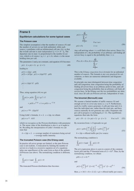
Frame 5<br />
Equilibrium calculations for some typical cases<br />
The Poisson case<br />
The simplest assumption is that the number of sources (N) and<br />
the number of servers (n) are both unlimited, while each<br />
source j contributes with an infinitesimal call rate (λj), so that<br />
the overall call rate is state independent λi = λ = N ⋅λj . The<br />
departure rate in state i is proportional to the number in service,<br />
which is of course i: µ i = i ⋅ µ= i/s, where s is the mean<br />
holding time per call.<br />
The parameters λ and µ are constants, and equation (43) becomes<br />
p(i) ⋅λ= p(i + 1) ⋅ µ ⋅ (i + 1) (48)<br />
leading to<br />
p(1) = (λ/µ) ⋅ p(0)<br />
p(2) = (λ/2µ) ⋅ p(1) = (λ/µ) 2 /2! ⋅ p(0)<br />
:<br />
:<br />
:<br />
p(i) = (λ/µ) i /i! ⋅ p(0)<br />
:<br />
:<br />
Thus, using equation (44) we get<br />
∞<br />
∑ p(i) = p(0)⋅ (λ / µ )<br />
i=0<br />
i<br />
∞<br />
∑ / i!<br />
i=0<br />
= p(0)⋅e λ / µ −λ / µ<br />
= 1 ⇒ p(0) = e<br />
and<br />
p(i) = e –λ/µ ⋅ (λ/µ) i /i!<br />
Using Little’s formula: A = λ ⋅ s = λ/µ, we obtain<br />
p(i) = e –A ⋅ Ai /i! (49)<br />
which we recognise as the Poisson distribution with parameter<br />
A. The mean value of the distribution is also A, as it ought to<br />
be. Recalling the interpretation of Little’s formula we can<br />
state that<br />
A = λ/µ = λ ⋅ s = average number of customers being served<br />
= average traffic intensity.<br />
The truncated Poisson case (the Erlang case)<br />
In practice all server groups are limited, so the pure Poisson<br />
case is not realistic. A truncation by limiting the number of<br />
servers to n leads to a recursive equation set of n equations<br />
(plus one superfluous) of the same form as that of the unlimited<br />
Poisson case above. The normalising condition is different,<br />
as<br />
n<br />
∞<br />
∑ p(i) = 1and ∑ p(i) = 0<br />
i=0<br />
i=n+1<br />
The truncated Poisson distribution thus becomes<br />
0 ≤ i ≤ n<br />
p(i) = 0, i > n<br />
(50)<br />
Any call arriving when i < n will find a free server. Since λ is<br />
independent of i, the probability of an arbitrary call finding all<br />
servers busy is equal to the probability that i = n:<br />
(51)<br />
This is the Erlang congestion (loss) formula for an unlimited<br />
number of sources. The formula is not very practical for calculations,<br />
so there are numerous tabulations and diagrams<br />
available.<br />
In principle one must distinguish between time congestion<br />
and call congestion, time congestion being the probability of<br />
finding all servers busy at an arbitrary point in time, and call<br />
congestion being the probability that an arbitrary call finds all<br />
servers busy. In the Erlang case the two probabilities are identical,<br />
since all calls are Poisson arrivals, independent of state.<br />
The binomial (Bernoulli) case<br />
We assume a limited number of traffic sources (N) and<br />
enough servers to cover any need, i.e. n ≥ N. Furthermore,<br />
each free traffic source generates λ calls per time unit (λ is<br />
here the individual rate, rather than the total rate, and busy<br />
sources naturally do not generate any calls). Departure rate<br />
per call in progress is unchanged µ = 1/s. The equilibrium<br />
equations then take the form<br />
p(i) ⋅ (N – i) ⋅ λ = p(i + 1) ⋅ µ ⋅ (i + 1) 0 ≤ i ≤ N (52)<br />
By recursion from i = 0 upwards we get<br />
p(i) = p(0)⋅<br />
b = λ/µ = offered traffic per free source<br />
N i<br />
⎛ ⎞ ⎛ λ ⎞<br />
⎝ i<br />
⋅<br />
⎠ ⎜ ⎟ = p(0)⋅<br />
⎝ µ ⎠<br />
N ⎛ ⎞<br />
⎝ i ⎠ ⋅bi<br />
The normalising condition is<br />
(53)<br />
The p(i)-expression above is seen to consist of the common<br />
factor p(0) and the ith binomial term of (1 + b) N . Thus, by the<br />
normalising condition, we obtain<br />
p(0) = (1 + b) –N<br />
and<br />
p(i) =<br />
P(n, A) = E(n, A) =<br />
N<br />
∞<br />
∑ p(i) = 1and ∑ p(i) = 0<br />
i=0<br />
i= N +1<br />
p(i) = N ⎛<br />
⎝ i<br />
A i<br />
i!<br />
A j<br />
n<br />
∑<br />
j =0<br />
j!<br />
⎞<br />
⎠ ⋅bi ⋅ 1+ b<br />
A n<br />
n!<br />
A j<br />
n<br />
∑<br />
j = 0<br />
j!<br />
( ) − N = N ⎛ ⎞<br />
⎝ i ⎠ ⋅ai N −i<br />
⋅( 1− a)<br />
Here, a = b/(1 + b) = λ /(λ + µ) = offered traffic per source.<br />
(54)


