Contents Telektronikk - Telenor

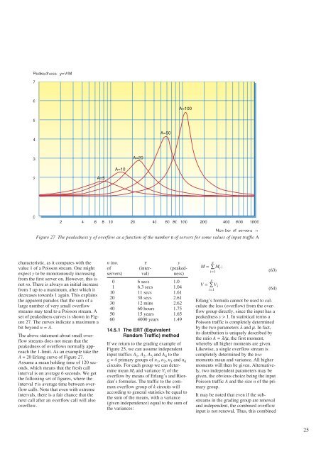
Peakedness: y=V/M
7
6
5
4
3
2
1
characteristic, as it compares with the
value 1 of a Poisson stream. One might
expect y to be monotonously increasing
from the first server on. However, this is
not so. There is always an initial increase
from 1 up to a maximum, after which it
decreases towards 1 again. This explains
the apparent paradox that the sum of a
large number of very small overflow
streams may tend to a Poisson stream. A
set of peakedness curves is shown in Figure
27. The curves indicate a maximum a
bit beyond n = A.
The above statement about small overflow
streams does not mean that the
peakedness of overflows normally approach
the 1-limit. As an example take the
A = 20 Erlang curve of Figure 27.
Assume a mean holding time of 120 seconds,
which means that the fresh call
interval is on average 6 seconds. We get
the following set of figures, where the
interval τ is average time between overflow
calls. Note that even with extreme
intervals, there is a fair chance that the
next call after an overflow call will also
overflow.
A=5
A=10
A=20
0
1 2 4 6 8 10 20 40 60 80 100 200 400 600 1000
Number of servers n
Figure 27 The peakedness y of overflow as a function of the number n of servers for some values of input traffic A
A=50
A=100
n (no. τ y
of (inter- (peakedservers)
val) ness)
0 6 secs 1.0
1 6.3 secs 1.04
10 11 secs 1.61
20 38 secs 2.61
30 12 mins 2.62
40 60 hours 1.75
50 15 years 1.65
60 4000 years 1.49
14.5.1 The ERT (Equivalent
Random Traffic) method
If we return to the grading example of
Figure 25, we can assume independent
input traffics A1 , A2 , A3 and A4 to the
g = 4 primary groups of n1 , n2 , n3 and n4 circuits. For each group we can determine
mean Mi and variance Vi of the
overflow by means of Erlang’s and Riordan’s
formulas. The traffic to the common
overflow group of k circuits will
according to general statistics be equal to
the sum of the means, with a variance
(given independence) equal to the sum of
the variances:
g
M = ∑ Mi ;
i=1
g
V = ∑Vi
i=1
(63)
(64)
Erlang’s formula cannot be used to calculate
the loss (overflow) from the overflow
group directly, since the input has a
peakedness y > 1. In statistical terms a
Poisson traffic is completely determined
by the two parameters λ and µ. In fact,
its distribution is uniquely described by
the ratio A = λ/µ, the first moment,
whereby all higher moments are given.
Likewise, a single overflow stream is
completely determined by the two
moments mean and variance. All higher
moments will then be given. Alternatively,
two independent parameters may be
given, the obvious choice being the input
Poisson traffic A and the size n of the primary
group.
It may be noted that even if the substreams
in the grading group are renewal
and independent, the combined overflow
input is not renewal. Thus, this combined
25