Intégration et Probabilités

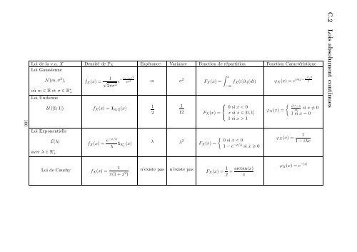
100Loi de la v.a. X Densité de P X Espérance Variance Fonction de répartition Fonction CaractéristiqueLoi GaussienneN(m,σ 2 ),où m ∈ R et σ ∈ R ∗ +1f X (x) = √2πσ 2 e−(x−m)2 2σ 2 m σ 2 ∫ xF X (x) = f X (t)λ 1 (dt)−∞ϕ X (x) = e imx− σ2 x 22Loi UniformeU ([0,1]) f X (x) = 1 [0,1] (x) 12Loi ExponentielleE(λ)avec λ ∈ R ∗ +1⎧⎨12 F X (x) =⎩0 si x < 0x si x ∈ [0,1]1 si x > 1{f X (x) = e−x/λλ 1 R ∗ (x) λ λ 2 0 si x < 0F+ X (x) =1 − e −x/λ si x 0ϕ X (x) =ϕ X (x) ={ e ix −1ixsi x ≠ 01 si x = 011 − iλxC.2 Lois absolument continuesLoi de Cauchy f X (x) =1π(1 + x 2 )n’existe pasn’existe pasF X (x) = 1 2 + arctan(x)πϕ X (x) = e −|x|