Annexe IV Modèle de Hubbard standard et états cohérents - Toubkal

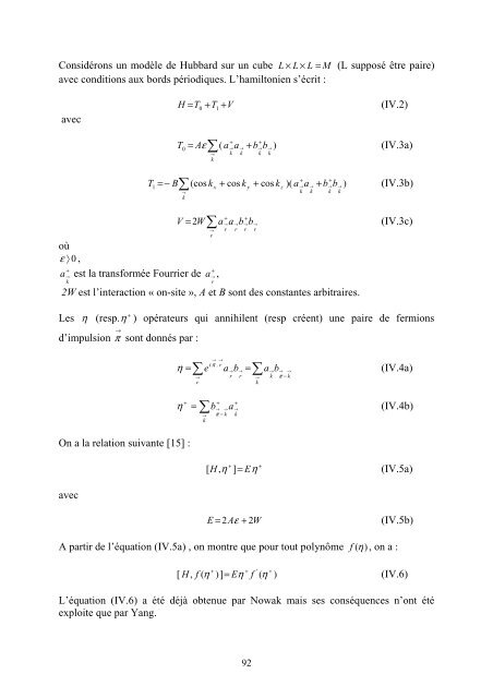
Considérons un modèle de Hubbard sur un cube L × L × L = M (L supposé être paire)avec conditions aux bords périodiques. L’hamiltonien s’écrit :avecH = T0 + T1+ V(IV.2)T0= Aε ( a a + b b )(IV.3a)∑→k+→k→k+→k→kT1= − B (cos k + cos k + cos k )( a a + b b ) (IV.3b)∑→kxyz+→k→k+→k→koùε 〉 0 ,+a est la transformée Fourrier de→kV = 2 W a a b b(IV.3c)∑→r+a ,2W est l’interaction « on-site », A et B sont des constantes arbitraires.→r+→r→r+→r→r+Les η (resp. η ) opérateurs qui annihilent (resp créent) une paire de fermionsd’impulsion → π sont donnés par :η =∑→re→ →.i π ra→rb→r=∑→ka→kb→ →−π k(IV.4a)+ +η + = b→→a→(IV.4b)∑→ π − k kkOn a la relation suivante [15] :avec[ H , η+ ] = Eη +(IV.5a)E = 2 Aε + 2W(IV.5b)A partir de l’équation (IV.5a) , on montre que pour tout polynôme f (η ) , on a :++ ' +[ H , f ( η )] = Eηf ( η )(IV.6)L’équation (IV.6) a été déjà obtenue par Nowak mais ses conséquences n’ont étéexploite que par Yang.92