- Page 1 and 2:
CRANFIELD UNIVERSITY GC CARVALHO AN
- Page 3 and 4:
ABSTRACT The aim of this work was t
- Page 5 and 6:
I dedicate this work to the memory
- Page 7 and 8:
FIGURES TABLES APPENDICES NOTATION
- Page 9 and 10:
3.3.2.1 Welding parameters generato
- Page 11 and 12:
References Further reading Appendic
- Page 13 and 14:
Figure 3.12 Offsets for weld start
- Page 15 and 16:
Figure 6.31 Voltage step input test
- Page 17 and 18:
Figure J. 2 Plot of stand-off varia
- Page 19 and 20:
Table A. 1 Welding extended entity
- Page 22 and 23:
NOTATION A, Electrode sectional are
- Page 24 and 25:
Pr(ign) Possibility measure of proc
- Page 26 and 27:
1. Introduction Welding is the thir
- Page 28:
Chapter 4 describes the on-line pos
- Page 31 and 32:
In pulse transfer, the welding curr
- Page 33 and 34:
Pd = Pv - pzh-s (2.1) where Pd is t
- Page 35 and 36:
the bridge. Another factor that ind
- Page 37 and 38:
establish the stable conditions for
- Page 39 and 40:
Philpott [ref. 21] developed an on-
- Page 41 and 42:
current peak at the moment the tip
- Page 43 and 44:
obot on the line must be individual
- Page 45 and 46:
collision detection capabilities wh
- Page 47 and 48:
cause dynamic variation in the seam
- Page 49 and 50:
Another type of robot static calibr
- Page 51 and 52:
spatter the gas nozzle is particula
- Page 53 and 54:
Table 2.1: Joint positioning tolera
- Page 55 and 56:
In order to minimise the undesirabl
- Page 57 and 58:
c) Ultrasonic sensors; d) Through-t
- Page 59 and 60:
where K,, K2, K3 and K4 are constan
- Page 61 and 62:
Philpott [refs. 21,131], based on t
- Page 63 and 64:
centre. This is attributed to the m
- Page 65 and 66:
technique must be employed to preve
- Page 67 and 68:
" digital hardware, which is basica
- Page 69 and 70:
" Maximum value, W.: Wmý = max(W )
- Page 71 and 72:
process studied over a small range.
- Page 73 and 74:
In-process welding control is a muc
- Page 75 and 76:
volume caused by the presence of a
- Page 77 and 78:
SHIELDING GAS IN CONSUMABLE ELECTRO
- Page 79 and 80:
Arc voltage Anode Arc length I Anod
- Page 81 and 82:
computed ideal procedure optimisnti
- Page 83 and 84:
CONSTANT CURRENT POWER SOURCE `j' O
- Page 85 and 86:
Original Surface New Surface Electr
- Page 87 and 88:
otating welding wire direction weld
- Page 89 and 90:
3.1.1.1 Robot errors A robot arm is
- Page 91 and 92:
3.2.2 Programming error correction
- Page 93 and 94:
3.3.2 Off-line programming module I
- Page 95 and 96:
Pen is the weld penetration (side p
- Page 97 and 98:
a. 2) Geometrical constraints from
- Page 99 and 100:
Step 11 Step 12 Step 13 Step 14 Ste
- Page 101 and 102:
Step 21 Step 22 If the wire feed sp
- Page 103 and 104: the Y'-axis results in a positive "
- Page 105 and 106: _ p1e0a - pORoba m31 Ilp! - poll (3
- Page 107 and 108: of a robot in its zero position12 w
- Page 109 and 110: frame points to the front of the ro
- Page 111 and 112: CAD Off-line (AutoCAD) programming
- Page 113 and 114: Z Surface 4 A Y 7 M2 Open Edge Join
- Page 115 and 116: WCF World Co-ordinates Frame 2a = J
- Page 117 and 118: x Torch Co-ordinates Frame o Indica
- Page 119 and 120: vo Ö 't7 Y7 't O m O 'S O O S O S
- Page 121 and 122: ýý aý 0 oA aW ö A O Zt A OO 't
- Page 123 and 124: Ti 9ý-! i4 *Tx t ap31 jx ý- ymin
- Page 125 and 126: errors', (i. e. joint positioning,
- Page 127 and 128: was considered to be outside the sc
- Page 129 and 130: Table 4.3 - Linguistic representati
- Page 131 and 132: The introduction of such a reduced
- Page 133 and 134: Table 4.8 - Final welding process c
- Page 135 and 136: the collection of welding data corr
- Page 137 and 138: Step 4- Calculate the confidence of
- Page 139 and 140: Z Table Co-ordinates Frame Y X Robo
- Page 141 and 142: 5.3 Monitoring system The monitorin
- Page 143 and 144: the torch end. Only one degree of f
- Page 145 and 146: Current: 500 Position: 234.5 5.7.3
- Page 147 and 148: I" va JI ºr ö C 3 r" r" rl f_ £-
- Page 149 and 150: IgurC a. H -I UI qur vCiSUJ JpCCU C
- Page 151 and 152: 126
- Page 153: Table 6.1 - Welding trials carried
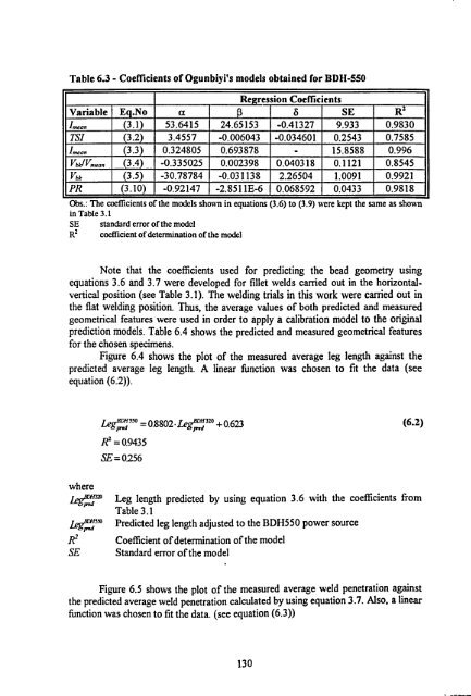
- Page 157 and 158: Note that the calibration model sho
- Page 159 and 160: Table 6.6 - Welding parameters used
- Page 161 and 162: constant set-up welding parameters
- Page 163 and 164: stickout lengths and the temperatur
- Page 165 and 166: of the dip mode of metal transfer.
- Page 167 and 168: which would become active by settin
- Page 169 and 170: In section 4.2.5 it has been mentio
- Page 171 and 172: 300 280 260 240 rd 35- 3D 25 20 15
- Page 173 and 174: Figure 6.5 - Measured "versus" Pred
- Page 175 and 176: i S 0 -0.1 -0.2 -0.3 -0.7- 68 10 12
- Page 177 and 178: 32.0 E 31.5 y 31.0 30.5 30.0 j 29.5
- Page 179 and 180: 35 - 30 p 15 10 0.00 2.60 5.42 8.23
- Page 181 and 182: 40 35 30 25 20 15 10 A+iIII+F0.17 2
- Page 183 and 184: 30 28 26 24 22 SO_act [mm] DipR [mo
- Page 185 and 186: 22 20 18 SO_act [mm] DipR [ohm/100]
- Page 187 and 188: !: 30 25 20t 10 5-- 0 Dip Transfer
- Page 189 and 190: 0.430- - 0.380- - :r 0.330 fPR L- 0
- Page 191 and 192: 7.2 Tests with varying stand-off an
- Page 193 and 194: Table 7.3 - Bead geometry along the
- Page 195 and 196: ö a2 ., u" u,.., g .,. aucyuaac VI
- Page 197 and 198: 0 24-- 22-- 18 210 1 90 0 v 170 mm
- Page 199 and 200: Q 34 32 3o mIm Viewing direction Fl
- Page 201 and 202: ýa 34 mm JO a .. ý nn ýr "u 00 M
- Page 203 and 204: 22 20 18 Viewing direction Flange W
- Page 205 and 206:
36 33 31 o 29 t 350 310 o 290 U due
- Page 207 and 208:
I C, x -i 23 21 j 19 Q 240c WFS =10
- Page 209 and 210:
en 34 32 - vsec 30- 26- 24 + .. ++
- Page 211 and 212:
186
- Page 213 and 214:
" to design and build the hardware
- Page 215 and 216:
Although only linear joints were im
- Page 217 and 218:
for predicting possibility of bad a
- Page 219 and 220:
8.4 Process monitoring and control
- Page 221 and 222:
satisfy the required quality criter
- Page 223 and 224:
198
- Page 225 and 226:
types of joints and multi-pass weld
- Page 227 and 228:
[14] NEMCHINSKY, V. A. The effect o
- Page 229 and 230:
[38] D1LTHEY, U. , REICHELL, T. , S
- Page 231 and 232:
[64] KING, F-J. and HIRSCH, P. Seam
- Page 233 and 234:
[86] CARGNELLI, M. and ROGOWSKI, A.
- Page 235 and 236:
[109] KURKIN, N. S. and DRIKKER, V.
- Page 237 and 238:
[130] USHIO, M. , LIU, W. , MAO, W.
- Page 239 and 240:
[151] DAVIS, A. R. Orr-line gap det
- Page 241 and 242:
[177] COOK, G. E. Feedback and adap
- Page 243 and 244:
[201] WON, Y. J. and CHO, H. S. A f
- Page 245 and 246:
220
- Page 247 and 248:
222
- Page 249 and 250:
wnum: local variable which defines
- Page 251 and 252:
Table A. 1 - continuation List item
- Page 253 and 254:
Imean = a2 + b2*WFS + c2*SO + d2*SO
- Page 255 and 256:
TCP2 number are also defined. The o
- Page 257 and 258:
f ROBSET. DAT: This file is created
- Page 259 and 260:
Figure C. 3 - Main dialogue box of
- Page 261 and 262:
Choose the set of welding parameter
- Page 263 and 264:
Water Cooling optic fibre bundle 0
- Page 265 and 266:
Figure E. 1 - Main graphical screen
- Page 267 and 268:
242
- Page 269 and 270:
Table G. 2 - Interface box external
- Page 271 and 272:
Robot ii Controller +24W CO . +24Vd
- Page 273 and 274:
248
- Page 275 and 276:
Table 1.1 - continuation Run Vpk M
- Page 277 and 278:
10- y =0.001ac 0 r. dSO [mm] $0 '10
- Page 279 and 280:
5.00- 0.00 y=0.0019x 1000 1500 2000
- Page 281 and 282:
Table J. 7 - Welding data collected
- Page 283 and 284:
Table J. 10 - Welding data collecte
- Page 285 and 286:
Table J. 13 - Welding data collecte
- Page 287 and 288:
20.00- 15. M y=0.0047x - 1.7922 10.
- Page 289 and 290:
Table J. 18 - Welding data collecte
- Page 291 and 292:
266
- Page 293 and 294:
Table K. 1- continuation Set-up par
- Page 295 and 296:
Table K. 1 - continuation Set-up pa
- Page 297 and 298:
Table K. 2 - continuation Set up pa
- Page 299 and 300:
Table K. 2 - Continuation Set-up pa
- Page 301 and 302:
Table K. 3 - Continuation Set-up pa
- Page 303:
Table K. 3 - Continuation Setup par