LIBRARY ı6ıul 0) - Cranfield University

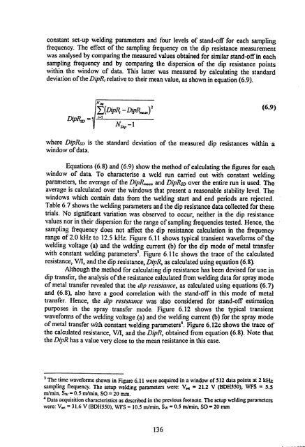
constant set-up welding parameters and four levels of stand-off for each sampling
frequency. The effect of the sampling frequency on the dip resistance measurement
was analysed by comparing the measured values obtained for similar stand-off in each
sampling frequency and by comparing the dispersion of the dip resistance points
within the window of data. This latter was measured by calculating the standard
deviation of the DipR, relative to their mean value, as shown in equation (6.9).
1N'
ThPR _ ; =1 ND,,
-1
(6.9)
where DipRSD is the standard deviation of the measured dip resistances within a
window of data.
Equations (6.8) and (6.9) show the method of calculating the figures for each
window of data. To characterise a weld run carried out with constant welding
parameters, the average of the DipR,
u,,, and DipRSD over the entire run is used. The
average is calculated over the windows that present a reasonable stability level. The
windows which contain data from the welding start and end periods are rejected.
Table 6.7 shows the welding parameters and the dip resistance data collected for these
trials. No significant variation was observed to occur, neither in the dip resistance
values nor in their dispersion for the range of sampling frequencies
tested. Hence, the
sampling frequency does not affect the dip resistance calculation in the frequency
range of 2.0 kHz to 12.5 kHz. Figure 6.11 shows typical transient waveforms of the
welding voltage (a) and the welding current (b) for the dip mode of metal transfer
with constant welding parameters3. Figure 6.11 c shows the trace of the calculated
resistance, V/I, and the dip resistance, DipR, as calculated using equation (6.8).
Although the method for calculating dip resistance has been devised for use in
dip transfer, the analysis of the resistance calculated from welding data for spray mode
of metal transfer revealed that the dip resistance, as calculated using equations (6.7)
and (6.8), also have a good correlation with the stand-off in this mode of metal
transfer. Hence, the dip resistance was also considered for stand-off estimation
purposes in the spray transfer mode. Figure 6.12 shows the typical transient
waveforms of the welding voltage (a) and the welding current (b) for the spray mode
of metal transfer with constant welding parameters". Figure 6.12c shows the trace of
the calculated resistance, V/1, and the DipR, obtained from equation (6.8). Note that
the DipR has a value very close to the mean resistance in this case.
3 The time waveforms shown in Figure 6.11 were acquired in a window of 512 data points at 2 kHz
sampling frequency. The setup welding parameters were: V., - 21.2 V (BDH550), WFS = 5.5
m/min, Sw = 0.5 m/min, SO = 20 mm.
Data acquisition characteristics as described in the previous footnote. The setup welding parameters
were: V,. t = 31.6 V (BDH550), WFS = 10.5 m/min, Sw - 0.5 m/min, SO - 20 mm
136