- Page 1 and 2: The Effects of CPAP Tube Reverse Fl
- Page 3 and 4: Acknowledgement First of all, I wou
- Page 5 and 6: When deep breathing induced reverse
- Page 7 and 8: 2.4.1 Reverse flow calculation ....
- Page 9 and 10: 5.3.1 Thermal dynamic model under s
- Page 11 and 12: XI.3 Steady state mask thermal bala
- Page 13 and 14: List of Figures Figure 1.1 Obstruct
- Page 15 and 16: Figure 5.10 Comparison between expe
- Page 17 and 18: Figure 6.13 Fluctuation of airflow
- Page 19 and 20: Table 5.3 Comparison of condensatio
- Page 21 and 22: Nomenclature Symbol Meaning of the
- Page 23 and 24: CMFeO CMFet C O C t Concentration o
- Page 25 and 26: m C 23 m Ca m cv m Cw m store m i m
- Page 27 and 28: Nu Cp Nu dir Nu Ti Nu To Nuwsn Nuws
- Page 29 and 30: QMor QMwst QTastn QTicn QTin Q
- Page 31 and 32: R Mic R Moc R Ticn R Toc R Torn Mas
- Page 33 and 34: V Capacity of the container m 3 V C
- Page 35 and 36: 1.1 Background Chapter 1 Introducti
- Page 37 and 38: The MRD is worn in user’s mouth w
- Page 39 and 40: Figure 1.4 CPAP machine Figure 1.5
- Page 41 and 42: 1.3 Literature survey A literature
- Page 43 and 44: CPAP fluid dynamic performance with
- Page 45 and 46: Chapter 2 Mathematical Modelling of
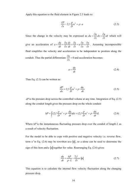
- Page 47: 2.3 Fluid dynamic analysis This sec
- Page 51 and 52: Figure 2.6 Pressure sensor - Honeyw
- Page 53 and 54: The pressure readings were taken af
- Page 55 and 56: Figure 2.12 Experimental set up for
- Page 57 and 58: 2.3.4 Chamber air space mass balanc
- Page 59 and 60: From the above analysis, the pressu
- Page 61 and 62: Figure 2.18 Full face mask and the
- Page 63 and 64: Inserting Eq. (2.26) and Eq. (2.27)
- Page 65 and 66: Where n( ) t is the airflow proper
- Page 67 and 68: However in reality, mixing turns ou
- Page 69 and 70: Chapter 3 Mathematical Modelling of
- Page 71 and 72: An Environment Control Chamber (Vö
- Page 73 and 74: Figure 3.4 Thermal enthalpy gain of
- Page 75 and 76: Figure 3.6 Heating element beneath
- Page 77 and 78: Figure 3.8 Chamber water heat balan
- Page 79 and 80: Table 3.1 Thermal resistance from h
- Page 81 and 82: 3.3.1.2 Heat balance at the outer s
- Page 83 and 84: 3.3.2 Heat flow from chamber water
- Page 85 and 86: through ADU which is a function of
- Page 87 and 88: It is assumed that the direct impac
- Page 89 and 90: Sc a a (3.47) Dwa Analogous to th
- Page 91 and 92: and keep them in gaseous status. On
- Page 93 and 94: through the walls and natural conve
- Page 95 and 96: Where d Ca is the specific humidity
- Page 97 and 98: TTa ( n1) is also considered as inl
- Page 99 and 100:
R Torn 2 2 ATlor ( TTWn T )( TTWn
- Page 101 and 102:
condensation severity but cannot ca
- Page 103 and 104:
condensation has occurred at all or
- Page 105 and 106:
The inlet is the air from HADT duri
- Page 107 and 108:
3.9 Average temperature of inhaled
- Page 109 and 110:
Table 4.1 Inputs to the fluid dynam
- Page 111 and 112:
Figure 4.2 Simulink TM model for fl
- Page 113 and 114:
Table 4.4 Outputs from the overall
- Page 115 and 116:
Gain block after input 1 is to conv
- Page 117 and 118:
Figure 4.7 Varying Transport Delay
- Page 119 and 120:
4.2.5 Mask mixing calculation subsy
- Page 121 and 122:
4.3 Computational model of thermal
- Page 123 and 124:
Figure 4.11 Block diagram of CPAP t
- Page 125 and 126:
Figure 4.13 Simulink TM model for t
- Page 127 and 128:
The outputs are listed in Table 4.1
- Page 129 and 130:
The outputs are listed in Table 4.1
- Page 131 and 132:
Figure 4.16 Dynamic chamber-air the
- Page 133 and 134:
Figure 4.17 HADT lump thermal balan
- Page 135 and 136:
Figure 4.18 Steady state HADT lump
- Page 137 and 138:
Figure 4.19 HADT lump air dynamic f
- Page 139 and 140:
The outputs are listed in Table 4.2
- Page 141 and 142:
Figure 4.21Steady state mask full t
- Page 143 and 144:
4 Temperature of airflow from HADT
- Page 145 and 146:
Average evaporation rate subsystem
- Page 147 and 148:
HADT and connects those upstream se
- Page 149 and 150:
The experiment was also carried out
- Page 151 and 152:
air flowing through the elbow, a ce
- Page 153 and 154:
expansion from the elbow to the mas
- Page 155 and 156:
Figure 5.12 Environmental control r
- Page 157 and 158:
Table 5.1 shows the combinations of
- Page 159 and 160:
Figure 5.17 Comparison of model out
- Page 161 and 162:
The comparison of experimental resu
- Page 163 and 164:
Figure 5.22 Comparison of model out
- Page 165 and 166:
Figure 5.24 Comparison of model out
- Page 167 and 168:
5.3.1.4 Airflow temperature at the
- Page 169 and 170:
flow rate had been even further inc
- Page 171 and 172:
Figure 5.31 Comparison of condensat
- Page 173 and 174:
Table 5.3 Comparison of condensatio
- Page 175 and 176:
3. The corrugated grooves on the HA
- Page 177 and 178:
5.3.2.1 Validation of evaporation r
- Page 179 and 180:
The experiment observation showed t
- Page 181 and 182:
Figure 6.1 Reverse flow under diffe
- Page 183 and 184:
It can also be seen in Figure 6.2 t
- Page 185 and 186:
within the same period. However, wh
- Page 187 and 188:
Figure 6.6 Comparison of evaporatio
- Page 189 and 190:
Figure 6.8 Airflow velocity in HADT
- Page 191 and 192:
Figure 6.11 Airflow velocity in HAD
- Page 193 and 194:
In Figure 6.14 the blue curve repre
- Page 195 and 196:
6.3.3.1.2 Comparison when heating e
- Page 197 and 198:
This vaporization potentiality (coi
- Page 199 and 200:
Figure 6.20 In-tube condensation of
- Page 201 and 202:
When using different sized masks, t
- Page 203 and 204:
Figure 6.23 Average specific humidi
- Page 205 and 206:
The average specific humidity in an
- Page 207 and 208:
Table 6.5 Comparison of average spe
- Page 209 and 210:
6. The deep breathing and reverse f
- Page 211 and 212:
Appendices Appendix I Regression of
- Page 213 and 214:
Appendix I. Regression of the press
- Page 215 and 216:
Figure I. 1 Tested results and the
- Page 217 and 218:
Appendix II. Regression of the pres
- Page 219 and 220:
Table III. 2 Airflow temperature an
- Page 221 and 222:
Appendix IV. The corrugated HADT ou
- Page 223 and 224:
The total area of the complicated c
- Page 225 and 226:
Figure V. 1 Regression of saturated
- Page 227 and 228:
This ratio can be regressed against
- Page 229 and 230:
Appendix VII. Details of the CPAP f
- Page 231 and 232:
VII.4 The mask pressure subsystem F
- Page 233 and 234:
Inputs to this water-centred subsys
- Page 235 and 236:
Input port number Input Unit 1 Heat
- Page 237 and 238:
input 4 is the portion of impact ar
- Page 239 and 240:
VIII.2.3 Water surface mass transfe
- Page 241 and 242:
This subsystem also contains two su
- Page 243 and 244:
VIII.2.5 Chamber wall 1 heat transf
- Page 245 and 246:
Figure VIII. 13 Wall 1 outer surfac
- Page 247 and 248:
Wall 2 and 3 inner surface temperat
- Page 249 and 250:
Figure VIII. 17 Chamber wall 2 and
- Page 251 and 252:
Inputs to this subsystem are listed
- Page 253 and 254:
Appendix IX. Details of steady stat
- Page 255 and 256:
Figure IX. 3 The HADT lump wall out
- Page 257 and 258:
Appendix X. Details of HADT lump ai
- Page 259 and 260:
2 Absolute value of airflow velocit
- Page 261 and 262:
Figure X. 5 HADT lump inlet absolut
- Page 263 and 264:
Figure XI. 2 Steady state mask mixi
- Page 265 and 266:
Figure XI. 4 Steady state mask wall
- Page 267 and 268:
Input port number Input Unit 1 Aver
- Page 269 and 270:
Appendix XII. Details of mask air d
- Page 271 and 272:
4 Length of the triangular plate in
- Page 273 and 274:
8 Length of the triangular plate in
- Page 275 and 276:
Appendix XIII. Details of the auxil
- Page 277 and 278:
XIII.3 Breath load average subsyste
- Page 279 and 280:
Figure XIII. 7 Average evaporation
- Page 281 and 282:
XIV.1.2 Under normal ambient temper
- Page 283 and 284:
XIV.2.3 Under high ambient temperat
- Page 285 and 286:
XIV.4 Airflow temperature at the en
- Page 287 and 288:
XIV.5.2 Under normal ambient temper
- Page 289 and 290:
XIV.6.3 Under high ambient temperat
- Page 291 and 292:
Appendix XVI. Regression of kinetic
- Page 293 and 294:
Figure XVII. 2 Condensation/evapora
- Page 295 and 296:
Figure XVIII. 2 Condensation/evapor
- Page 297 and 298:
at point C. Right after that, here
- Page 299 and 300:
Appendix XIX. Coefficient and param
- Page 301 and 302:
Average water thermal conductivity
- Page 303 and 304:
Appendix XXI. Fluid dynamic and the
- Page 305 and 306:
The lung simulator drives the air.
- Page 307 and 308:
Appendix XXII. Model user instructi
- Page 309 and 310:
The input blocks and their values a
- Page 311 and 312:
Dynamically fluctuating air tempera
- Page 313 and 314:
References [1] Good sleep advice. W
- Page 315 and 316:
[28] Schettino GPP, Chatmongkolchar
- Page 317:
[60] Marek R, Straub J. Analysis of