Statistics for Decision- Making in Business - Maricopa Community ...

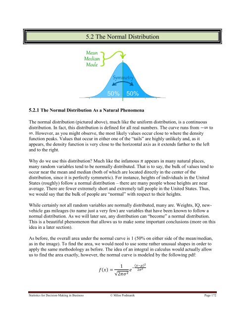
5.2 The Normal Distribution
5.2.1 The Normal Distribution As a Natural Phenomena
The normal distribution (pictured above), much like the uniform distribution, is a continuous
distribution. In fact, this distribution is defined for all real numbers. The curve runs from to
. However, as you might observe, the most likely values occur close to where the density
function peaks. Values that occur in either one of the “tails” are highly unlikely and, as it
appears, the density function is very close to the horizontal axis as it extends farther to the left
and to the right.
Why do we use this distribution Much like the infamous appears in many natural places,
many random variables tend to be normally distributed. That is to say, the bulk of values tend to
occur near the mean and median (both of which are located directly in the center of the
distribution, since it is perfectly symmetric). For instance, heights of individuals in the United
States (roughly) follow a normal distribution – there are many people whose heights are near
average. There are fewer extremely short and extremely tall people in the United States. Thus,
we would say that the bulk of people are “normal” with respect to their heights.
While certainly not all random variables are normally distributed, many are. Weights, IQ, newvehicle
gas mileages (to name just a very few) are variables that have been known to follow a
normal distribution. As we will later see, any distribution can “become” a normal distribution.
This is a beautiful phenomenon that allows us to make some important conclusions (more on this
idea in a later section).
As before, the overall area under the normal curve is 1 (50% on either side of the mean/median,
as in the image). To find the area, we would need to use some rather unusual shapes in order to
apply the same methodology as before. The idea of an integral in calculus would actually allow
us to find the area exactly, however, the normal curve is modeled by the following pdf:
( )
√
( )
Statistics for Decision-Making in Business © Milos Podmanik Page 172