Familia de Mapas del Panadero Como Ambiente Caótico de la ...

CAPÍTULO 5. CAMINATA ACOPLADA A PANADERO 58
distancia variacional clásica
distancia variacional clásica
1.4
1.3
1.2
1.1
1.0
0.9
0.8
0.7
0.6
0.5
0.4
0.3
0.2
0.1
0.0
B (Baker)
6,1
B
6,2
B
6,3
B
6,4
B
6,5
B (Many Coins)
6,6
0 20 40 60 80 100 120
t
140 160 180 200 220 240
1.8
1.6
1.4
1.2
1.0
0.8
0.6
0.4
0.2
1 qubit
2 qubits
3 qubits
4 qubits
5 qubits
6 qubits
7 qubits
0.0
0 20 40 60 80 100 120 140 160 180 200 220 240
t
Distancia Variacional Clásica
distancia variacional clásica
1.5
1.4
1.3
1.2
1.1
1.0
0.9
0.8
0.7
0.6
fam 1 (Baker)
fam 2
0.5
fam 3
0.4
fam 4
0.3
fam 5
0.2
fam 6
0.1
0.0
fam 7 (Many Coins)
0 20 40 60 80 100 120 140
t
160 180 200 220 240
1.8
1.7
1.6
1.5
1.4
1.3
1.2
1.1
1.0
0.9
0.8
0.7
0.6
2 qubits
3 qubits
0.5
4 qubits
0.4
5 qubits
0.3
6 qubits
0.2
0.1
0.0
7 qubits
0 20 40 60 80 100 120 140 160 180 200 220 240
t
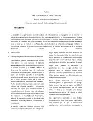
Figura 5.4: Distancia variacional clásica del caminante acoplado al panadero en la línea infinita para
la familia de 6 qubits y 7 qubits (arriba); y para varias monedas independientes y el mapa del panadero
convencional (abajo). En todos los casos el caminante se encontraba localizado en posición y el estado
inicial del panadero era el “simétrico”.
5.5. Varianza
Como ya vimos en el capítulo de la caminata cuántica, la varianza del caminante es una de
las medidas que nos permite analizar su comportamiento.
Todos los cálculos en este capítulo se realizarán para el caminante en la línea infinita con
estado inicial localizado en posición.
Podemos notar en la figura 5.3 que a tiempo cortos (del orden de
log 2(N) = ♯ qubits) la caminata clásica y los miembros de la familia de la caminata acoplada al
panadero se comportan de manera similar en distribución de probabilidades. Esto también se
puede apreciar en la varianza donde para todos los caminantes se obtiene un comportamiento
de tipo √ t.
A partir de cierto tiempo el comportamiento de la varianza es linael para todos los caminantes
cuánticos.