Reviews in Computational Chemistry Volume 18

More documents

Recommendations

Info

176 Charge-Transfer Reactions in Condensed Phases Optical excitations quite often generate considerable changes in fixed partial charges, usually described in terms of the difference solute dipole m0 (‘‘0’’ refers here to the solute). Chromophores with high magnitudes of the ratio m0=R 3 0 , where R0 is the effective solute radius, are often used as optical probes of the local solvent structure and solvation power. 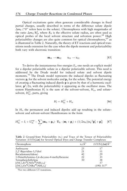68 High polarizability changes are also quite common for optical chromophores, 69 as is illustrated in Table 2. Naturally, the theory of ET reactions and optical transitions needs extension for the case when the dipole moment and polarizability both vary with electronic transition: m01 ! m02 a01 ! a02 ½85Š To derive the instantaneous free energies Ei, one needs an explicit model for a dipolar polarizable solute in a dipolar polarizable solvent. This need is addressed by the Drude model for induced solute and solvent dipole moments. 70 The Drude model represents the induced dipoles as fluctuating vectors: p j for the solvent molecules and p 0 for the solute. The potential energy of creating a fluctuating induced dipole p is given by that of a harmonic oscillator, p 2 =2a, with the polarizability a appearing as the oscillator mass. The system Hamiltonian Hi is the sum of the solvent–solvent, Hss, and solute– solvent, H ðiÞ 0s , parts, giving Hi ¼ H ðiÞ 0s þ Hss ½86Š In Hi, the permanent and induced dipoles add up resulting in the solute– solvent and solvent–solvent Hamiltonians in the form H ðiÞ 0s ¼ Ii þ U rep 0s X j ðm0i þ p0Þ T0j ðmj þ pjÞþð1=2a0iÞ½o 2 0 _p2 0 þ p20 Š ½87Š Table 2 Ground-State Polarizability (a1) and Trace of the Tensor of Polarizability Variation (1/3)Tr[ a] for Several Optical Dyes and Charge Transfer Complexes Chromophore a1/A˚ 3 (1/3)Tr[ a]/A˚ 3 Anthracene 25 17 2,20-Bipyridine-3,30diol 21 11 Bis(adamantylidene) 42 29 1-Dimethylamino-2,6-dicyano-4-methylbenzene 22 35 Tetraphenylethylene 50 38 [(NC)5Fe II CNOs III (NH3)5] [(NC)5Os 57 II CNRu III (NH3)5] (190) 317 a a For two different CT transitions.
and Hss ¼ U rep ss 1 2 X j;k ðmj þ p jÞ ~T jk ðm k þ p kÞþ 1 2a X j ½o 2 e _p 2 j þ p2 j Š ½88Š Here, Tjk is the dipole–dipole interaction tensor, and ~T jk ¼ Tjkð1 djkÞ; U rep 0s and Urep ss stand for repulsion potentials, and o0 ¼ E12=h, where E12 is the adiabatic gas-phase energy gap (Eq. [29]). The statistical average over the electronic degrees of freedom in Eq. [15] is equivalent, in the Drude model, to integration over the induced dipole moments p0 and pj. The Hamiltonian Hi is quadratic in the induced dipoles, and the trace can be calculated exactly as a functional integral over the fluctuating fields p0 and pj. 39,67 The resulting solute–solvent interaction energy is 67 E0s;i ¼ Ii þ U rep 0s þ Udisp 0s;i aefeim 2 0i feim0i Rp 1 2 a0ifeiR 2 p Here, Rp is the reaction field of the solvent nuclear subsystem, and the factor fei ¼ ½12aea0iŠ 1 describes an enhancement of the condensed-phase solute dipole and polarizability by the self-consistent field of the electronic polarization of the solvent. For the statistical average over the nuclear configurations, generating the distribution over the solute energy gaps (Eq. [18]), one needs to specify the fluctuation statistics of the nuclear reaction field Rp. A Gaussian statistics of the field fluctuations 35 implies using the distribution function ½89Š ½90Š PðRpÞ ¼ 4p apkBT 1=2 exp½ b R 2 p =4apŠ ½91Š where ap is the response coefficient of the nuclear solvent response. Combined with the Gaussian function PðRpÞ, Eq. [89] is essentially equivalent to the Q model (Eq. [65]). The vector of the nuclear reaction field plays the role of the nuclear collective mode driving activated transitions (q). One can then directly employ the results of the Q model to produce the diabatic free energy surfaces of polarizable donor–acceptor complexes or to calculate the spectroscopic observables. The reorganization energies follow from Eq. [71] and take the following form for polarizable chromophores: li ¼ðapfi=feiÞ ~m0 þ 2apfi ~a0m0i Beyond the Parabolas 177 2 ½92Š
Page 1 and 2:
Reviews in Computational Chemistry
Page 3 and 4:
Kenny B. Lipkowitz Department of Ch
Page 5 and 6:
vi Preface three-dimensional struct
Page 7 and 8:
viii Preface some descriptors and i
Page 9 and 10:
Epilogue and Dedication My associat
Page 11 and 12:
Contents 1. Clustering Methods and
Page 13 and 14:
Contents xv Electron Transfer in Po
Page 15 and 16:
Contributors John M. Barnard, Barna
Page 17 and 18:
Contributors to Previous Volumes *
Page 19 and 20:
Volume 3 (1992) Tamar Schlick, Opti
Page 21 and 22:
Volume 7 (1996) Geoffrey M. Downs a
Page 23 and 24:
Volume 11 (1997) Mark A. Murcko, Re
Page 25 and 26:
T. Daniel Crawford* and Henry F. Sc
Page 27 and 28:
Topics Covered in Volumes 1-18 * Ab
Page 29 and 30:
Reviews in Computational Chemistry
Page 31 and 32:
2 Clustering Methods and Their Uses
Page 33 and 34:
Page 35 and 36:
Page 37 and 38:
Page 39 and 40:
10 Clustering Methods and Their Use
Page 41 and 42:
Page 43 and 44:
Page 45 and 46:
Page 47 and 48:
Page 49 and 50:
Page 51 and 52:
Page 53 and 54:
Page 55 and 56:
Page 57 and 58:
Page 59 and 60:
Page 61 and 62:
Page 63 and 64:
Page 65 and 66:
Page 67 and 68:
Page 69 and 70:
Page 71 and 72:
42 The Use of Scoring Functions in
Page 73 and 74:
Page 75 and 76:
Page 77 and 78:
Page 79 and 80:
Table 1 Reference List for the Most
Page 81 and 82:
Page 83 and 84:
Page 85 and 86:
Page 87 and 88:
Page 89 and 90:
Page 91 and 92:
Page 93 and 94:
Page 95 and 96:
Page 97 and 98:
Page 99 and 100:
Page 101 and 102:
Page 103 and 104:
Page 105 and 106:
Page 107 and 108:
Page 109 and 110:
Page 111 and 112:
Page 113 and 114:
Page 115 and 116:
Page 117 and 118:
CHAPTER 3 Potentials and Algorithms
Page 119 and 120:
Vn (1 + cos(nω + γ)) 2 K θ (θ
Page 121 and 122:
are modified by their environment w
Page 123 and 124:
Table 1 Polarizability Parameters f
Page 125 and 126:
The polarizable point dipole models
Page 127 and 128:
two to three orders of magnitude sl
Page 129 and 130:
M i z i + q i d i k i and shell cha
Page 131 and 132:
Shell Models 103 on estimates of sh
Page 133 and 134:
minimization can be replaced by mor
Page 135 and 136:
The energy required to create a cha
Page 137 and 138:
for all i ði:e:; 8 iÞ: @U @qi l
Page 139 and 140:
where we have used q Cl ¼ qNa. The
Page 141 and 142:
Electronegativity Equalization Mode
Page 143 and 144:
Electronegativity Equalization Mode
Page 145 and 146:
of N molecules is taken as a Hartre
Page 147 and 148:
is treated using variable charges.
Page 149 and 150:
water have been developed, includin
Page 151 and 152:
Applications 123 classical and rigi
Page 153 and 154: developing polarizable models. A va
Page 155 and 156: Comparison of the Polarization Mode
Page 157 and 158: negligible errors in such propertie
Page 159 and 160: ecome significant at field strength
Page 161 and 162: noteworthy in this regard because t
Page 163 and 164: References 135 9. P. Cieplak and P.
Page 165 and 166: References 137 48. E. L. Pollock an
Page 167 and 168: References 139 Computational Chemis
Page 169 and 170: References 141 139. J. Hinze and H.
Page 171 and 172: References 143 178. J. J. P. Stewar
Page 173 and 174: References 145 216. M. W. Mahoney a
Page 175 and 176: CHAPTER 4 New Developments in the T
Page 177 and 178: Introduction 149 applications). For
Page 179 and 180: FCWD(∆E ) FCWD(0) ∆E = 0 ∆E
Page 181 and 182: Introduction 153 Equations [6]-[12]
Page 183 and 184: Paradigm of Free Energy Surfaces 15
Page 185 and 186: Paradigm of Free Energy Surfaces 15
Page 187 and 188: In Eqs. [18] and [19], F0i is the e
Page 189 and 190: where ‘‘þ’’ and ‘‘ ’
Page 191 and 192: is, however, small for the usual co
Page 193 and 194: solute-solvent coupling through the
Page 195 and 196: where Z is the electrode overpotent
Page 197 and 198: energy surfaces of ET. 33,50-56 It
Page 199 and 200: This result indicates a fundamental
Page 201 and 202: βF i (X ) 40 20 0 −20 1 2 βλ 1
Page 203: Table 1 Main Features of the Two-Pa
Page 207 and 208: λ i /eV 4 3 2 1 0 0 10 20 30 40 Bo
Page 209 and 210: the width/Stokes shift relation (Eq
Page 211 and 212: Table 3 Mapping of the Q Model on S
Page 213 and 214: This situation is of course not sat
Page 215 and 216: F ± (Y ad )/λ I 0.8 0.4 0 −0.4
Page 217 and 218: it by choosing the GMH basis set 7
Page 219 and 220: Anharmonic higher order terms gain
Page 221 and 222: of the radiation is the perturbatio
Page 223 and 224: individual vibrational excitations
Page 225 and 226: m 12 /D 6 5.5 5 4.5 4 3.5 17 18 19
Page 227 and 228: In Eq. [144], the coordinates Y km
Page 229 and 230: ε/M −1 cm −1 4000 2000 0 analy
Page 231 and 232: βσ 2 /10 3 cm −1 14 12 10 8 Opt
Page 233 and 234: 0.2 0.1 0 12 16 20 24 28 32 The app
Page 235 and 236: References 207 7. M. D. Newton, Adv
Page 237 and 238: References 209 59. R. Kubo and Y. T
show all

Reviews in Computational Chemistry Volume 18

Create successful ePaper yourself

Delete template?

Save as template?