- Page 1 and 2:
Reviews in Computational Chemistry
- Page 3 and 4:
Kenny B. Lipkowitz Department of Ch
- Page 5 and 6:
vi Preface three-dimensional struct
- Page 7 and 8:
viii Preface some descriptors and i
- Page 9 and 10:
Epilogue and Dedication My associat
- Page 11 and 12:
Contents 1. Clustering Methods and
- Page 13 and 14:
Contents xv Electron Transfer in Po
- Page 15 and 16:
Contributors John M. Barnard, Barna
- Page 17 and 18:
Contributors to Previous Volumes *
- Page 19 and 20:
Volume 3 (1992) Tamar Schlick, Opti
- Page 21 and 22:
Volume 7 (1996) Geoffrey M. Downs a
- Page 23 and 24:
Volume 11 (1997) Mark A. Murcko, Re
- Page 25 and 26:
T. Daniel Crawford* and Henry F. Sc
- Page 27 and 28:
Topics Covered in Volumes 1-18 * Ab
- Page 29 and 30:
Reviews in Computational Chemistry
- Page 31 and 32:
2 Clustering Methods and Their Uses
- Page 33 and 34:
4 Clustering Methods and Their Uses
- Page 35 and 36:
6 Clustering Methods and Their Uses
- Page 37 and 38:
8 Clustering Methods and Their Uses
- Page 39 and 40:
10 Clustering Methods and Their Use
- Page 41 and 42:
12 Clustering Methods and Their Use
- Page 43 and 44:
14 Clustering Methods and Their Use
- Page 45 and 46:
16 Clustering Methods and Their Use
- Page 47 and 48:
18 Clustering Methods and Their Use
- Page 49 and 50:
20 Clustering Methods and Their Use
- Page 51 and 52:
22 Clustering Methods and Their Use
- Page 53 and 54:
24 Clustering Methods and Their Use
- Page 55 and 56:
26 Clustering Methods and Their Use
- Page 57 and 58:
28 Clustering Methods and Their Use
- Page 59 and 60:
30 Clustering Methods and Their Use
- Page 61 and 62:
32 Clustering Methods and Their Use
- Page 63 and 64:
34 Clustering Methods and Their Use
- Page 65 and 66:
36 Clustering Methods and Their Use
- Page 67 and 68:
38 Clustering Methods and Their Use
- Page 69 and 70:
40 Clustering Methods and Their Use
- Page 71 and 72:
42 The Use of Scoring Functions in
- Page 73 and 74:
44 The Use of Scoring Functions in
- Page 75 and 76:
46 The Use of Scoring Functions in
- Page 77 and 78:
48 The Use of Scoring Functions in
- Page 79 and 80:
Table 1 Reference List for the Most
- Page 81 and 82:
52 The Use of Scoring Functions in
- Page 83 and 84:
54 The Use of Scoring Functions in
- Page 85 and 86:
56 The Use of Scoring Functions in
- Page 87 and 88:
58 The Use of Scoring Functions in
- Page 89 and 90:
60 The Use of Scoring Functions in
- Page 91 and 92:
62 The Use of Scoring Functions in
- Page 93 and 94:
64 The Use of Scoring Functions in
- Page 95 and 96:
66 The Use of Scoring Functions in
- Page 97 and 98:
68 The Use of Scoring Functions in
- Page 99 and 100:
70 The Use of Scoring Functions in
- Page 101 and 102:
72 The Use of Scoring Functions in
- Page 103 and 104:
74 The Use of Scoring Functions in
- Page 105 and 106:
76 The Use of Scoring Functions in
- Page 107 and 108:
78 The Use of Scoring Functions in
- Page 109 and 110:
80 The Use of Scoring Functions in
- Page 111 and 112:
82 The Use of Scoring Functions in
- Page 113 and 114:
84 The Use of Scoring Functions in
- Page 115 and 116:
86 The Use of Scoring Functions in
- Page 117 and 118:
CHAPTER 3 Potentials and Algorithms
- Page 119 and 120:
Vn (1 + cos(nω + γ)) 2 K θ (θ
- Page 121 and 122:
are modified by their environment w
- Page 123 and 124:
Table 1 Polarizability Parameters f
- Page 125 and 126:
The polarizable point dipole models
- Page 127 and 128:
two to three orders of magnitude sl
- Page 129 and 130:
M i z i + q i d i k i and shell cha
- Page 131 and 132:
Shell Models 103 on estimates of sh
- Page 133 and 134:
minimization can be replaced by mor
- Page 135 and 136:
The energy required to create a cha
- Page 137 and 138:
for all i ði:e:; 8 iÞ: @U @qi l
- Page 139 and 140:
where we have used q Cl ¼ qNa. The
- Page 141 and 142:
Electronegativity Equalization Mode
- Page 143 and 144:
Electronegativity Equalization Mode
- Page 145 and 146:
of N molecules is taken as a Hartre
- Page 147 and 148:
is treated using variable charges.
- Page 149 and 150:
water have been developed, includin
- Page 151 and 152:
Applications 123 classical and rigi
- Page 153 and 154:
developing polarizable models. A va
- Page 155 and 156: Comparison of the Polarization Mode
- Page 157 and 158: negligible errors in such propertie
- Page 159 and 160: ecome significant at field strength
- Page 161 and 162: noteworthy in this regard because t
- Page 163 and 164: References 135 9. P. Cieplak and P.
- Page 165 and 166: References 137 48. E. L. Pollock an
- Page 167 and 168: References 139 Computational Chemis
- Page 169 and 170: References 141 139. J. Hinze and H.
- Page 171 and 172: References 143 178. J. J. P. Stewar
- Page 173 and 174: References 145 216. M. W. Mahoney a
- Page 175 and 176: CHAPTER 4 New Developments in the T
- Page 177 and 178: Introduction 149 applications). For
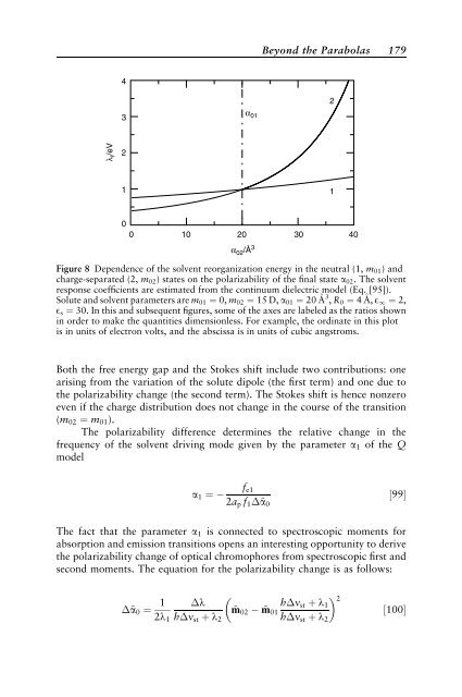
- Page 179 and 180: FCWD(∆E ) FCWD(0) ∆E = 0 ∆E
- Page 181 and 182: Introduction 153 Equations [6]-[12]
- Page 183 and 184: Paradigm of Free Energy Surfaces 15
- Page 185 and 186: Paradigm of Free Energy Surfaces 15
- Page 187 and 188: In Eqs. [18] and [19], F0i is the e
- Page 189 and 190: where ‘‘þ’’ and ‘‘ ’
- Page 191 and 192: is, however, small for the usual co
- Page 193 and 194: solute-solvent coupling through the
- Page 195 and 196: where Z is the electrode overpotent
- Page 197 and 198: energy surfaces of ET. 33,50-56 It
- Page 199 and 200: This result indicates a fundamental
- Page 201 and 202: βF i (X ) 40 20 0 −20 1 2 βλ 1
- Page 203 and 204: Table 1 Main Features of the Two-Pa
- Page 205: and Hss ¼ U rep ss 1 2 X j;k ðmj
- Page 209 and 210: the width/Stokes shift relation (Eq
- Page 211 and 212: Table 3 Mapping of the Q Model on S
- Page 213 and 214: This situation is of course not sat
- Page 215 and 216: F ± (Y ad )/λ I 0.8 0.4 0 −0.4
- Page 217 and 218: it by choosing the GMH basis set 7
- Page 219 and 220: Anharmonic higher order terms gain
- Page 221 and 222: of the radiation is the perturbatio
- Page 223 and 224: individual vibrational excitations
- Page 225 and 226: m 12 /D 6 5.5 5 4.5 4 3.5 17 18 19
- Page 227 and 228: In Eq. [144], the coordinates Y km
- Page 229 and 230: ε/M −1 cm −1 4000 2000 0 analy
- Page 231 and 232: βσ 2 /10 3 cm −1 14 12 10 8 Opt
- Page 233 and 234: 0.2 0.1 0 12 16 20 24 28 32 The app
- Page 235 and 236: References 207 7. M. D. Newton, Adv
- Page 237 and 238: References 209 59. R. Kubo and Y. T