Baltic Sea

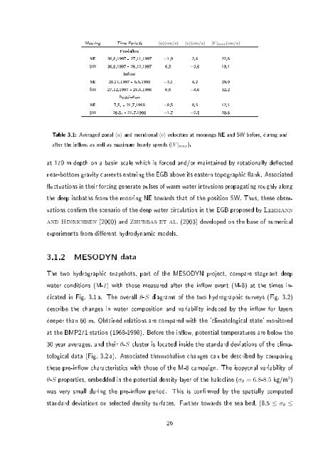
Mooring Time Periods 〈u〉(cm/s) 〈v〉(cm/s) |V | max(cm/s)
Pre-inow
NE 30.8.1997 - 27.11.1997 −1.9 2.4 22.6
SW 30.8.1997 - 26.12.1997 0.5 −3.0 19.1
Inow
NE 28.11.1997 - 6.5.1998 −3.1 4.2 29.0
SW 27.12.1997 - 25.5.1998 0.9 −4.0 32.2
Post-inow
NE 7.5. - 21.7.1998 −0.5 0.3 12.1
SW 26.5. - 21.7.1998 −1.7 −2.5 20.6
Table 3.1: Averaged zonal 〈u〉 and meridional 〈v〉 velocities at moorings NE and SW before, during and
after the inow, as well as maximum hourly speeds (|V | max ).
at 170 m depth on a basin scale which is forced and/or maintained by rotationally deected
near-bottom gravity currents entering the EGB above its eastern topographic ank. Associated
uctuations in their forcing generate pulses of warm water intrusions propagating roughly along
the deep isobaths from the mooring NE towards that of the position SW. Thus, these observations
conrm the scenario of the deep water circulation in the EGB proposed by Lehmann
and Hinrichsen (2000) and Zhurbas et al. (2003) developed on the base of numerical
experiments from dierent hydrodynamic models.
3.1.2 MESODYN data
The two hydrographic snapshots, part of the MESODYN project, compare stagnant deep
water conditions (M-7) with those measured after the inow event (M-8) at the times indicated
in Fig. 3.1 a. The overall θ-S diagrams of the two hydrographic surveys (Fig. 3.2)
describe the changes in water composition and variability induced by the inow for layers
deeper than 60 m. Obtained relations are compared with the 'climatological state' monitored
at the BMP271 station (1968-1998). Before the inow, potential temperatures are below the
30 year averages, and their θ-S cluster is located inside the standard deviations of the climatological
data (Fig. 3.2 a). Associated thermohaline changes can be described by comparing
these pre-inow characteristics with those of the M-8 campaign. The isopycnal variability of
θ-S properties, embedded in the potential density layer of the halocline (σ θ = 6.8-8.5 kg/m 3 )
was very small during the pre-inow period. This is conrmed by the spatially computed
standard deviations on selected density surfaces. Further towards the sea bed, (8.5 ≤ σ θ ≤
26