Baltic Sea

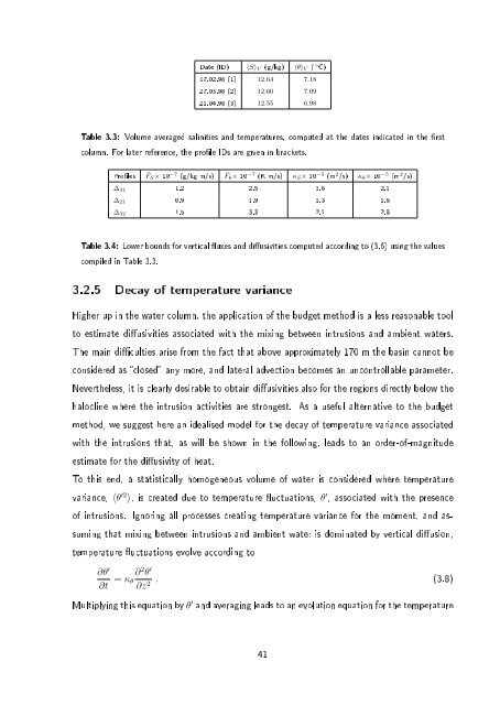
Date (ID) 〈S〉 V (g/kg) 〈θ〉 V ( ◦ C)
17.02.98 (1) 12.64 7.18
27.03.98 (2) 12.60 7.09
21.04.98 (3) 12.55 6.98
Table 3.3: Volume averaged salinities and temperatures, computed at the dates indicated in the rst
column. For later reference, the prole IDs are given in brackets.
Proles ¯FS × 10 −7 (g/kg m/s) ¯Fθ × 10 −7 (K m/s) κ S × 10 −5 (m 2 /s) κ θ × 10 −5 (m 2 /s)
∆ 31 1.2 2.5 1.6 2.1
∆ 21 0.9 1.9 1.3 1.6
∆ 32 1.5 3.3 2.1 2.8
Table 3.4: Lower bounds for vertical uxes and diusivities computed according to (3.6) using the values
compiled in Table 3.3.
3.2.5 Decay of temperature variance
Higher up in the water column, the application of the budget method is a less reasonable tool
to estimate diusivities associated with the mixing between intrusions and ambient waters.
The main diculties arise from the fact that above approximately 170 m the basin cannot be
considered as closed any more, and lateral advection becomes an uncontrollable parameter.
Nevertheless, it is clearly desirable to obtain diusivities also for the regions directly below the
halocline where the intrusion activities are strongest. As a useful alternative to the budget
method, we suggest here an idealised model for the decay of temperature variance associated
with the intrusions that, as will be shown in the following, leads to an order-of-magnitude
estimate for the diusivity of heat.
To this end, a statistically homogeneous volume of water is considered where temperature
variance, 〈θ ′2 〉, is created due to temperature uctuations, θ ′ , associated with the presence
of intrusions. Ignoring all processes creating temperature variance for the moment, and assuming
that mixing between intrusions and ambient water is dominated by vertical diusion,
temperature uctuations evolve according to
∂θ ′
∂t = κ ∂ 2 θ ′
θ
∂z . (3.8)
2
Multiplying this equation by θ ′ and averaging leads to an evolution equation for the temperature
41