Analysis and Ranking of the Acoustic Disturbance Potential of ...

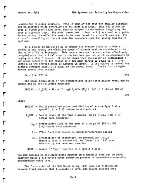
Report No. 6945
BBN Systems and Technologies Corporation
reaches the cruising altitude. This is usually not true for smaller aircraft
and helicopters which generally fly at lower altitudes. Thus the effective
area of significant sound level near an airport is determined largely by the
type of aircraft used. The model described in Section 4.3 was used as a guide
in estimating the effective areas to be considered for aircraft sources. For
aircraft travelling at low altitude the procedure used for moving sources is
applied .
If a source is moving so as to change its average location within a
period of two hours, the effective speed of advance must be considered since
the value of Pe is increa ed. This occurs because the source has effectively
occupied more than a 1 km 5 area in the two hour period, which is equivalent to
ha ing more than 1 source. It can be shown that the number of independent 1
km
3 areas occupied by the source in a two-hour period is equal to (1+1.77S)
where S is the average speed of advance in km/hr. If the source is travelling
along a straight path, S is equal to the actual speed. The Pe for a single
moving source then becomes
The basic formulation of the Standardized Noise Contribution Model can be
summarized by the following equation:
SNC(S1) = Ls(S1) - TLr + 10 Log{(Tf)(Pe)(Ns)} (dB re 1 pPa at 300 m)
where
SNC(S1) = The standardized noise contribution of source Type 1 at a
specific site (1/3 octave band spectrum)
L,(SI) = Source Level of the Type 1 source (dB re 1 wPa, 1 m) (1/3
octave band spectrum)
TLr = Transmission Loss in the area at a range of 300 m (dB)
(1/3 octave band spectrum)
Tf = (Time Fraction) Source-on duration/Reference period
Pe = (Probability of Encounter) The probability that a
specific type of source will be found in a 1 km2 area
surrounding the receiver location
N(S1) = Number of Type 1 sources in a specific area.
The SNC spectra of the significant sources in a specific area can be added
together using a 1/3 octave power summation process to determine a composite
standardized noise level.
The formulation of the SNC Model in Eq. (20) does not distinguish
between fixed sources that fluctuate in level and moving sources that