recent developments in high frequency financial ... - Index of

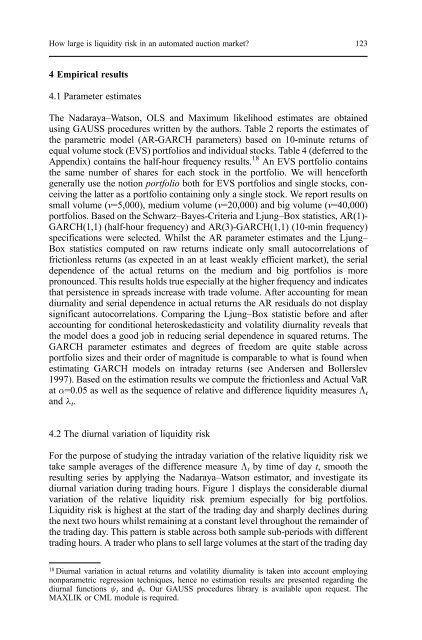
How large is liquidity risk in an automated auction market? 123
4 Empirical results
4.1 Parameter estimates
The Nadaraya–Watson, OLS and Maximum likelihood estimates are obtained
using GAUSS procedures written by the authors. Table 2 reports the estimates of
the parametric model (AR-GARCH parameters) based on 10-minute returns of
equal volume stock (EVS) portfolios and individual stocks. Table 4 (deferred to the
Appendix) contains the half-hour frequency results. 18 An EVS portfolio contains
the same number of shares for each stock in the portfolio. We will henceforth
generally use the notion portfolio both for EVS portfolios and single stocks, conceiving
the latter as a portfolio containing only a single stock. We report results on
small volume (v=5,000), medium volume (v=20,000) and big volume (v=40,000)
portfolios. Based on the Schwarz–Bayes-Criteria and Ljung–Box statistics, AR(1)-
GARCH(1,1) (half-hour frequency) and AR(3)-GARCH(1,1) (10-min frequency)
specifications were selected. Whilst the AR parameter estimates and the Ljung–
Box statistics computed on raw returns indicate only small autocorrelations of
frictionless returns (as expected in an at least weakly efficient market), the serial
dependence of the actual returns on the medium and big portfolios is more
pronounced. This results holds true especially at the higher frequency and indicates
that persistence in spreads increase with trade volume. After accounting for mean
diurnality and serial dependence in actual returns the AR residuals do not display
significant autocorrelations. Comparing the Ljung–Box statistic before and after
accounting for conditional heteroskedasticity and volatility diurnality reveals that
the model does a good job in reducing serial dependence in squared returns. The
GARCH parameter estimates and degrees of freedom are quite stable across
portfolio sizes and their order of magnitude is comparable to what is found when
estimating GARCH models on intraday returns (see Andersen and Bollerslev
1997). Based on the estimation results we compute the frictionless and Actual VaR
at α=0.05 as well as the sequence of relative and difference liquidity measures Λt
and t.
4.2 The diurnal variation of liquidity risk
For the purpose of studying the intraday variation of the relative liquidity risk we
take sample averages of the difference measure Λ t by time of day t, smooth the
resulting series by applying the Nadaraya–Watson estimator, and investigate its
diurnal variation during trading hours. Figure 1 displays the considerable diurnal
variation of the relative liquidity risk premium especially for big portfolios.
Liquidity risk is highest at the start of the trading day and sharply declines during
the next two hours whilst remaining at a constant level throughout the remainder of
the trading day. This pattern is stable across both sample sub-periods with different
trading hours. A trader who plans to sell large volumes at the start of the trading day
18 Diurnal variation in actual returns and volatility diurnality is taken into account employing
nonparametric regression techniques, hence no estimation results are presented regarding the
diurnal functions t and t. Our GAUSS procedures library is available upon request. The
MAXLIK or CML module is required.