

recent developments in high frequency financial ... - Index of
recent developments in high frequency financial ... - Index of
recent developments in high frequency financial ... - Index of

You also want an ePaper? Increase the reach of your titles
YUMPU automatically turns print PDFs into web optimized ePapers that Google loves.
Exchange rate volatility and the mixture <strong>of</strong> distribution hypothesis 11<br />
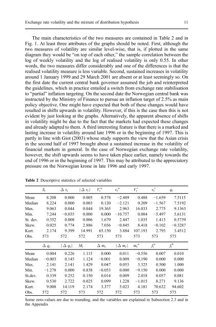
The ma<strong>in</strong> characteristics <strong>of</strong> the two measures are conta<strong>in</strong>ed <strong>in</strong> Table 2 and <strong>in</strong><br />
Fig. 1. At least three attributes <strong>of</strong> the graphs should be noted. First, although the<br />
two measures <strong>of</strong> volatility are similar level-wise, that is, if plotted <strong>in</strong> the same<br />
diagram they would be “on top <strong>of</strong> each other,” the sample correlation between the<br />
log <strong>of</strong> weekly volatility and the log <strong>of</strong> realised volatility is only 0.55. In other<br />
words, the two measures differ considerably and one <strong>of</strong> the differences is that the<br />
realised volatility measure is less variable. Second, susta<strong>in</strong>ed <strong>in</strong>creases <strong>in</strong> volatility<br />
around 1 January 1999 and 29 March 2001 are absent or at least seem<strong>in</strong>gly so. On<br />
the first date the current central bank governor assumed the job and re<strong>in</strong>terpreted<br />
the guidel<strong>in</strong>es, which <strong>in</strong> practice entailed a switch from exchange rate stabilisation<br />
to “partial” <strong>in</strong>flation target<strong>in</strong>g. On the second date the Norwegian central bank was<br />
<strong>in</strong>structed by the M<strong>in</strong>istry <strong>of</strong> F<strong>in</strong>ance to pursue an <strong>in</strong>flation target <strong>of</strong> 2.5% as ma<strong>in</strong><br />
policy objective. One might have expected that both <strong>of</strong> these changes would have<br />
resulted <strong>in</strong> shifts upwards <strong>in</strong> volatility. However, if this is the case then this is not<br />
evident by just look<strong>in</strong>g at the graphs. Alternatively, the apparent absence <strong>of</strong> shifts<br />
<strong>in</strong> volatility might be due to the fact that the markets had expected these changes<br />
and already adapted to them. A third <strong>in</strong>terest<strong>in</strong>g feature is that there is a marked and<br />
last<strong>in</strong>g <strong>in</strong>crease <strong>in</strong> volatility around late 1996 or <strong>in</strong> the beg<strong>in</strong>n<strong>in</strong>g <strong>of</strong> 1997. This is<br />
partly <strong>in</strong> l<strong>in</strong>e with Giot (2003) whose study supports the view that the Asian crisis<br />
<strong>in</strong> the second half <strong>of</strong> 1997 brought about a susta<strong>in</strong>ed <strong>in</strong>crease <strong>in</strong> the volatility <strong>of</strong><br />
f<strong>in</strong>ancial markets <strong>in</strong> general. In the case <strong>of</strong> Norwegian exchange rate volatility,<br />
however, the shift upwards seems to have taken place earlier, namely towards the<br />
end <strong>of</strong> 1996 or <strong>in</strong> the beg<strong>in</strong>n<strong>in</strong>g <strong>of</strong> 1997. This may be attributed to the appreciatory<br />
pressure on the Norwegian krone <strong>in</strong> late 1996 and early 1997.<br />
Table 2 Descriptive statistics <strong>of</strong> selected variables<br />
S t Δ s t ∣Δ s t∣ V t w<br />
Mean 8.208 0.000 0.005 0.578 −2.489 0.488 −1.659 7.5115<br />
Median 8.224 0.000 0.003 0.120 −2.121 0.209 −1.567 7.5192<br />
Max. 9.063 0.044 0.044 19.365 2.963 16.033 2.775 9.1363<br />
M<strong>in</strong>. 7.244 −0.035 0.000 0.000 −10.757 0.004 −5.497 5.6131<br />
St. dev. 0.352 0.008 0.006 1.679 2.447 1.035 1.413 0.5739<br />
Skew. 0.025 0.774 2.886 7.036 −0.845 8.418 −0.102 −0.3287<br />
Kurt. 2.174 9.399 14.991 65.150 3.884 107.193 2.793 3.4512<br />
Obs. 573 572 572 573 573 573 573 573<br />
v t w<br />
Δ qt ∣Δ qt∣ Mt Δ mt ∣Δ mt∣ mt w<br />
Mean 0.004 0.226 1.115 0.000 0.011 −0.556 0.007 0.010<br />
Median −0.003 0.145 1.124 −0.001 0.009 −0.190 0.000 0.000<br />
Max. 2.141 2.141 1.429 0.047 0.053 3.325 0.500 1.000<br />
M<strong>in</strong>. −1.278 0.000 0.838 −0.053 0.000 −9.150 0.000 0.000<br />
St.dev. 0.339 0.252 0.150 0.014 0.009 2.018 0.057 0.081<br />
Skew. 0.530 2.722 0.025 0.099 1.228 −1.015 8.271 9.136<br />
Kurt. 9.008 14.119 2.174 3.377 5.023 4.181 70.632 94.602<br />
Obs. 572 572 573 572 572 573 573 573<br />
Some zero-values are due to round<strong>in</strong>g, and the variables are expla<strong>in</strong>ed <strong>in</strong> Subsection 2.3 and <strong>in</strong><br />
the Appendix<br />
V t r<br />
v t r<br />
ft a<br />
q t<br />
ft b


