recent developments in high frequency financial ... - Index of

236 J. M. Rodríguez-Poo et al.
certain threshold. We define the threshold as $0.125. Following Engle and Russell (1998),
the price is defined as the mid-quote. A volume duration is defined as the time interval
needed to observe an accumulated change in volume greater than a given number of
shares. The threshold is defined to be 25,000 shares. The data sample covers September,
October, and November 1996, and the stocks are Boeing for price durations and Disney
for volume durations. The choice of these two stocks and its time horizon is motivated
by the fact that Bauwens et al. (2004) show, in a density forecast analysis, that they are
difficult to model, both in terms of expectation and density.
Price and volume durations provide an instantaneous overview of two important market
features. Price durations are strongly linked to the instantaneous volatility process,
see Engle and Russell (1998) and Gerhard and Hautsch (2002). By computing the conditional
expectation of the duration, it is possible to compute the instantaneous volatility
process. Volume durations are appealing as they convey information about two of the
three dimensions of the liquidity: time and volume. Therefore, price and volume durations
provide measures of the instantaneous volatility and the liquidity of the market.
Prior to estimation we follow Engle and Russell (1998) and two transformations are
performed: (1) Trades and bid/ask quotes recorded before 09:30 am and after 4 pm are
ignored and (2) the time gaps between market closing and opening and weekends are also
ignored.
3.2 Descriptive analysis
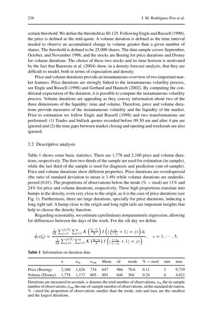
Table 1 shows some basic statistics. There are 1,778 and 2,160 price and volume durations,
respectively. The first two-thirds of the sample are used for estimation (in-sample),
while the last third of the sample is used for diagnosis and prediction (out-of-sample).
Price and volume durations show different properties. Price durations are overdispersed
(the ratio of standard deviation to mean is 1.49) while volume durations are underdispersed
(0.81). The proportions of observations below the mode (% < mod) are 11% and
24% for price and volume durations, respectively. These high proportions translate into
humps in the density, even very close to the origin, as it is the case of price durations (see
Fig. 1). Furthermore, there are large durations, specially for price durations, inducing a
long right tail. A hump close to the origin and long right tails are important insights that
help to choose the density function.
Regarding seasonality, we estimate a preliminary nonparametric regression, allowing
for differences between the days of the week. For the sth day we define
ˆφs(t ′ 0 ) =
1
nh
1
nh
�⌊n/5⌋ �ni=1 j=1 K
� ⌊n/5⌋
j=1
Table 1 Information on duration data
� t ′ 0 −t ′ i
h
�ni=1 K � � t0−ti
h I
� �
I ⌊ t−to
�
+ 1⌋=js di
tc−to
�
⌊ t−to
� , s = 1, ··· , 5,
+ 1⌋=js
tc−to
n nin nout Mean sd mode % < mod min max
Price (Boeing) 2,160 1,426 734 647 966 70.6 0.11 3 9,739
Volume (Disney) 1,778 1,173 605 801 648 304 0.24 6 4,621
Durations are measured in seconds. n denotes the total number of observations, nin the in-sample
number of observations,nout the out-of-sample number of observations, sd the standard deviation,
%