recent developments in high frequency financial ... - Index of

A multivariate integer count hurdle model 45
The unconditional bivariate histogram of the simulated time series is presented
in Fig. 9. Although the positive dependence between the marginal processes is
reflected, the shape of the histogram does not correspond to the empirical one
in full (see Fig. 1). In particular the frequency of the outcome (0, 0) has been
considerably underestimated. We compute the differences between the histograms
of the empirical and the simulated data to infer in which points (i,j) the observed
and the estimated probabilities disagree. To assess these differences graphically,
we plotted in Fig. 10 only positive differences and in Fig. 11 only absolute negative
differences. Besides the outcome probability of (0, 0), the probabilities for points
(i,j) concentrated around (0,0) are a little bit underestimated (positive differences
in Fig. 10) as well, and the probabilities for points (i,j) which are a little further
away from (0,0) are a little overestimated (negative differences in Fig. 11). Thus,
we conclude that we underestimate the kurtosis of the empirical distribution. The
real data is much more concentrated in the outcome (0,0), as well as evidencing
much fatter tails. There is a clear signal for a tail dependency in the data generating
process, as the extreme positive or negative movements of the exchange rates take
place much more often than could be explained by a standard Gaussian copula
function (see Fig. 10).
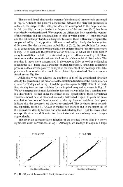
Additionally, we can address the goodness-of-fit of the conditional bivariate
density by considering the bivariate autocorrelation function of the residual series
ˆεt = (ˆε 1 t , ˆε2 t )′ depicted in Fig. 14 and the quantile–quantile (QQ) plots of the modified
density forecast test variables for the implied marginal processes in Fig. 12.
We have mapped these modified density forecast test variables into a standard normal
distribution, so that under the correct model specification, these normalized
variables should be i.i.d. standard normally distributed. Figure 13 plots the autocorrelation
functions of these normalized density forecast variables. Both plots
indicate that the processes are almost uncorrelated. The deviation from normality,
especially for the EUR/USD exchange rate changes and in the upper tail of
the normalized density forecast variables indicated by the QQ-plots, reveals that
our specification has difficulties to characterize extreme exchange rate changes
appropriately.
The bivariate autocorrelation function of the residual series (Fig. 14) shows
significant cross-correlations at lag 1. Although, we manage to explain a large
Empirical Qunatiles
−5 −3 −1 1 2 3 4 5
−4
EUR/GBP EUR/USD
Empirical Qunatiles
−5 −3 −1 1 2 3 4 5
−2 0 1 2 3 4 5 −4
Std. Normal Quantiles
Fig. 12 QQ plot of the normalized density forecast variables.
−2 0 1 2 3 4 5
Std. Normal Quantiles