sin αst

LIST OF ATTACHMENTSSTRUCTURAL ANALYSIS OF BLADES
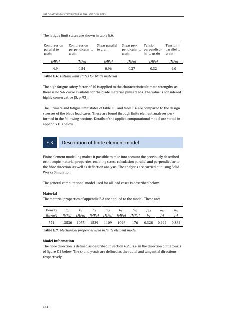
The fatigue limit states are shown in table E.6.
Compression
parallel to
grain
152
[MPa]
Compression
perpendicular to
grain
[MPa]
Shear parallel
to grain
[MPa]
Shear perpendicular
to
grain
[MPa]
Tension
perpendicular
to grain
[MPa]
Tension
parallel to
grain
[MPa]
4.9 0.54 0.96 0.27 0.32 9.0
Table E.6: Fatigue limit states for blade material
The high fatigue safety factor of 10 is applied to the characteristic ultimate strengths, as
there is no S-N curve available for the blade material, pinus taeda. The value is considered
highly conservative [5, p. 93].
The ultimate and fatigue limit states of table E.5 and table E.6 are compared to the design
stresses of the blade load cases. These are found through finite element analyses per-
formed in the following sections. Details of the applied computational model are stated in
appendix E.3 below.
E.3 Description of finite element model
Finite element modelling makes it possible to take into account the previously described
orthotropic material properties, enabling stress calculation parallel and perpendicular to
the fibre direction, as well as deflection analysis. The analyses are carried out using Solid-
Works Simulation.
The general computational model used for all load cases is described below.
Material
The material properties of appendix E.2 are applied to the model. These are:
Density
[kg/m 3]
EL
[MPa]
ET
[MPa]
ER
[MPa]
GLR
[MPa]
GLT
[MPa]
GRT
[MPa]
571 13530 1055 1529 1109 1096 176 0.328 0.292 0.382
Table E.7: Mechanical properties used in finite element model
Model information
The fibre direction is defined as described in section 6.2.3, i.e. in the direction of the z-axis
of figure E.2 below. The x- and y-axis are defined as the radial and tangential directions,
respectively.
�LR
[-]
�LT
[-]
�RT
[-]