GUIDE WAVE ANALYSIS AND FORECASTING - WMO

Probability of non-exceedance
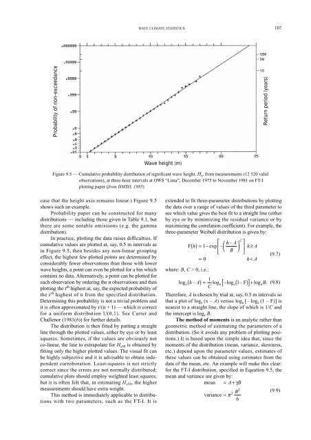
case that the height axis remains linear.) Figure 9.5
shows such an example.
Probability paper can be constructed for many
distributions — including those given in Table 9.1, but
there are some notable omissions (e.g. the gamma
distribution).
In practice, plotting the data raises difficulties. If
cumulative values are plotted at, say, 0.5 m intervals as
in Figure 9.5, then besides any non-linear grouping
effect, the highest few plotted points are determined by
considerably fewer observations than those with lower
wave heights, a point can even be plotted for a bin which
contains no data. Alternatively, a point can be plotted for
each observation by ordering the n observations and then
plotting the r th highest at, say, the expected probability of
the r th highest of n from the specified distribution.
Determining this probability is not a trivial problem and
it is often approximated by r/(n + 1) — which is correct
for a uniform distribution U(0,1). See Carter and
Challenor (1981(b)) for further details.
The distribution is then fitted by putting a straight
line through the plotted values, either by eye or by least
squares. Sometimes, if the values are obviously not
co-linear, the line to extrapolate for H s50 is obtained by
fitting only the higher plotted values. The visual fit can
be highly subjective and it is advisable to obtain independent
corroboration. Least-squares is not strictly
correct since the errors are not normally distributed;
cumulative plots should employ weighted least squares,
but it is often felt that, in estimating H s50, the higher
measurements should have extra weight.
This method is immediately applicable to distributions
with two parameters, such as the FT-I. It is
WAVE CLIMATE STATISTICS 107
Wave height (m)
Figure 9.5 — Cumulative probability distribution of significant wave height, H s, from measurements (12 520 valid
observations), at three-hour intervals at OWS “Lima”, December 1975 to November 1981 on FT-I
plotting paper (from HMSO, 1985)
Return period (years)
extended to fit three-parameter distributions by plotting
the data over a range of values of the third parameter to
see which value gives the best fit to a straight line (either
by eye or by minimizing the residual variance or by
maximizing the correlation coefficient). For example, the
three-parameter Weibull distribution is given by:
(9.7)
where: B, C > 0, i.e.:
(9.8)
Therefore, A is chosen by trial at, say, 0.5 m intervals so
that a plot of loge (x – A) versus loge [– loge (1 – F)] is
nearest to a straight line, the slope of which is 1/C and
the intercept is loge B.
The method of moments is an analytic rather than
geometric method of estimating the parameters of a
distribution. (So it avoids any problem of plotting positions.)
It is based upon the simple idea that, since the
moments of the distribution (mean, variance, skewness,
etc.) depend upon the parameter values, estimates of
these values can be obtained using estimates from the
data of the mean, etc. An example will make this clear:
for the FT-I distribution, specified in Equation 9.5, the
mean and variance are given by:
mean = A+ γB
B
(9.9)
variance = π 2
C ⎡ h A
F( h)
= −
⎛ – ⎞ ⎤
1 exp ⎢–
h A
⎝ B ⎠
⎥ ≥
⎣ ⎦
= 0
h< A
1
loge( h– A)
= loge[ – loge( 1–
F) ]+ logeB.
C
2
6