GUIDE WAVE ANALYSIS AND FORECASTING - WMO

32
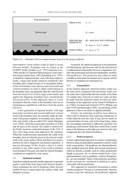
Free atmosphere
Ekman layer
Constant flux layer
representative ocean surface winds as input to ocean
forecast models. Examples may be found in the
ECMWF model (Tiedtke, et al., 1979; Simmons et al.,
1988) and the US National Meteorological Center spectral
forecast model (Sela, 1982; Kanamitsu et al., 1991).
It should be emphasized that, even with these improvements,
a large-scale model cannot be considered a true
boundary-layer model because of its incomplete formulation
of boundary-layer physics and horizontal and
vertical resolution. In order to obtain wind forecasts in
the boundary layer, one generally takes the wind forecast
from the lowest level of these large-scale models and
applies the diagnostic boundary-layer considerations
discussed earlier. In this approach, there is a tacit
assumption that the winds in the boundary layer are in
instantaneous equilibrium with those from the model
first level.
A new generation of regional models, with high
horizontal resolution and several additional vertical
levels in the boundary layer, are currently under development
with greater emphasis on boundary-layer physics.
One such model is the so-called ETA model (Mesinger
et al., 1988), which has a horizontal resolution of 20 km
and 40 layers in the vertical. The model is centred over
the North American continental domain of the USA. It
also covers large ocean areas adjacent to the continent.
When this model becomes operational, the winds in the
boundary layer are directly given by the forecast model
itself at the ocean surface (20 m) and there is no need to
perform the above diagnostic calculations separately. A
special advantage of this model is that it is easily
portable to any other region of the world to produce
meteorological forecasts, provided the lateral boundary
conditions are supplied by some means.
2.5 Statistical methods
Statistical methods provide another approach to generate
surface wind fields from large-scale forecast models.
These techniques do well in situations where forecast
models do not or cannot depict the surface winds with
adequate accuracy.
GUIDE TO WAVE ANALYSIS AND FORECASTING
(above 1 km)
Matched layer
(below 50 m)
Ocean surface
Figure 2.10 — Schematic of the two-regime boundary layer, K is the mixing coefficient
u = G
K = const.
ρK = du/dz, du/dz, and u continuous
K = κu * z, κ = 0.4, τ = const.
(z = z 0 ), u * , u = 0
In general, the statistical approach to the generation
of wind analyses and forecasts calls for the derivation of
a mathematical relationship between a dependent variable
(the predictand) and selected independent variables
(the predictors). The predictors may either be made
available to forecasters for manual use or may be entered
directly to computers for automated use.
2.5.1 Extrapolation
In the simplest approach, observed surface winds over
the land can be compared with concurrent winds over
the water and a relationship derived, usually in the form
of a simple ratio. Forecasts of wind over water can then
be made from the projected values of wind over land.
Examples of this approach can be found in Richards et
al. (1966), Overland and Gemmill (1977), Phillips and
Irbe (1978) and Burroughs (1984). An advantage of this
approach is that it can easily be applied manually.
Clearly, the technique would be most effective
when used in situations only requiring estimations of
winds relatively near the coast. It may also be useful on
enclosed bodies of water, such as the Great Lakes, where
the surrounding wind field is sufficiently specified. For
producing wind forecast fields that extend from coastal
areas to far distances on the high seas, however, this type
of approach has only limited usefulness.
2.5.2 Perfect prognosis
A more sophisticated approach is to derive a relationship
between analysed atmospheric parameters and the winds
at the ocean surface. The predictors are obtained directly
from gridded analysed fields and include parameters
which are directly available, such as winds, geopotential
height or pressure, etc. at various model levels. Computed
parameters such as gradients, vorticity, divergence,
etc. are also included. Values of the predictors anywhere
on the grid may be considered in addition to values
collocated with the predictand.
This approach to statistical forecasting is called
“perfect prognosis” because it is assumed that, when the
scheme is put into operation, the predictors supplied