GUIDE WAVE ANALYSIS AND FORECASTING - WMO

60
it may also be dissipated through interaction with the
sea-bed (bottom friction). More details are given in
Sections 3.4 and 7.6.
5.4.4 Non-linear interactions
Generally speaking, any strong non-linearities in the
wave field and its evolution are accounted for in the
dissipation terms. Input and dissipation terms can be
regarded as complementary to those linear and weakly
non-linear aspects of the wave field which we are able to
describe dynamically. Into this category fall the propagation
of surface waves and the redistribution of energy
within the wave spectrum due to weak, non-linear interactions
between wave components, which is designated
as a source term, Snl. The non-linear interactions are
discussed in Section 3.5.
The effect of the term, Snl, is briefly as follows: in
the dominant region of the spectrum near the peak, the
wind input is greater than the dissipation. The excess
energy is transferred by the non-linear interactions
towards higher and lower frequencies. At the higher
frequencies the energy is dissipated, whereas the transfer
to lower frequencies leads to growth of new wave
components on the forward (left) side of the spectrum.
This results in migration of the spectral peak towards
lower frequencies. The non-linear wave-wave interactions
preserve the spectral shape and can be calculated
exactly.
The source term Snl can be handled exactly but the
requirement on computing power is great. In third generation
models, the non-linear interactions between wave
components are indeed computed explicitly by use of
special integration techniques and with the aid of simplifications
introduced by Hasselmann and Hasselmann
(1985) and Hasselmann et al. (1985). Even with these
simplifications powerful computers are required to
produce real-time wave forecasts. Therefore many
second generation models are still in operational use. In
second generation numerical wave models, the nonlinear
interaction is parameterized or treated in a
simplified way. This may give rise to significant differences
between models. A simplified illustration of the
∆y
j+2
j+1
j
j-1
i-1
θ0
(x0, y0) (x0, y0)
GUIDE TO WAVE ANALYSIS AND FORECASTING
θ0 θ
i i+1 i+2
∆x
three source terms in relation to the wave spectrum is
shown in Figure 3.7.
5.4.5 Propagation
Wave energy propagates not at the velocity of the waves
or wave crests (which is the phase velocity: the speed at
which the phase is constant) but at the group velocity
(see Section 1.3.2). In wave modelling we are dealing
with descriptors such as the energy density and so it is
the group velocity which is important.
The propagative effects of water waves are quantified
by noting that the local rate of change of energy is
equal to the net rate of flow of energy to or from that
locality, i.e. the divergence of energy-density flux. The
practical problem encountered in computer modelling is
to find a numerical scheme for calculating this. In
manual models, propagation is only considered outside
the generation area and attention is focused on the
dispersion and spreading of waves as they propagate.
Propagation affects the growth of waves through
the balance between energy leaving a locality and that
entering it. In a numerical model it is the propagation of
wave energy which enables fetch-limited growth to be
modelled. Energy levels over land are zero and so downwind
of a coast there is no upstream input of wave
energy. Hence energy input from the atmosphere is propagated
away, keeping total energy levels near the coast
low.
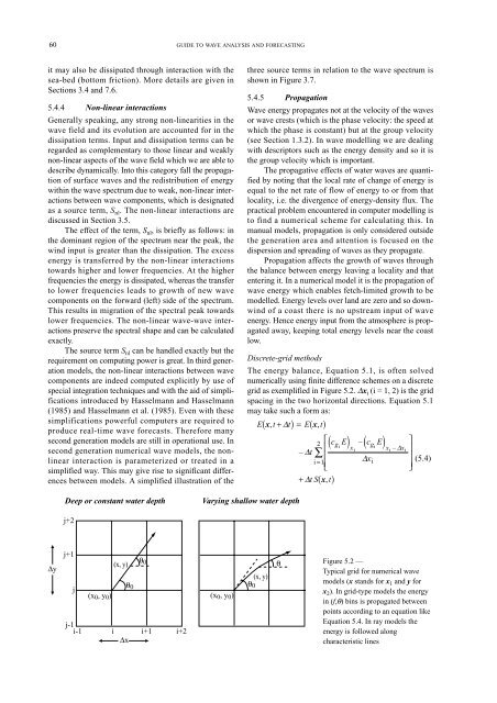
Discrete-grid methods
The energy balance, Equation 5.1, is often solved
numerically using finite difference schemes on a discrete
grid as exemplified in Figure 5.2. ∆xi (i = 1, 2) is the grid
spacing in the two horizontal directions. Equation 5.1
may take such a form as:
E x, t+ ∆t
E x,
t
(x, y)
θ0
( ) = ( )
Deep or constant water depth Varying shallow water depth
(x, y)
( ) ( )
⎡ E – E ⎤
2 cgc ⎢ i g
x i
i xi – ∆xi
⎥
– ∆t
∑ ⎢
⎥ (5.4)
i= 1 ∆x
⎣
⎢
i
⎦
⎥
∆tS
x,
t
+ ( )
Figure 5.2 —
Typical grid for numerical wave
models (x stands for x 1 and y for
x 2). In grid-type models the energy
in (f,θ) bins is propagated between
points according to an equation like
Equation 5.4. In ray models the
energy is followed along
characteristic lines