GUIDE WAVE ANALYSIS AND FORECASTING - WMO

More documents

Recommendations

Info

42 Energy, E (m 2 /Hz) Application of the source terms is not always straightforward. The theoretical-empirical mix in most wave models allows for some “tuning” of the models. This also depends on the grid, the boundary configuration, the type of input winds, the time-step, the influence of depth, computer power available, etc. Manual methods, on the other hand, conform to what may be regarded as fairly universal rules and can usually be applied anywhere without modification. For manual calculations, the distinction between wind sea and swell is quite real and an essential part of the computation process. For the hybrid parametric models (see Chapter 5) it is necessary, although the problem of interfacing the wind-wave and swell regimes arises. For numerical models which use spectral components for all the calculations (i.e. discrete spectral models) the definition of swell is quite arbitrary. 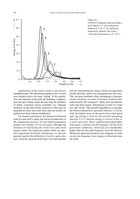From the spectrum alone there is no hard and fast 4 3 GUIDE TO WAVE ANALYSIS AND FORECASTING 0.7 Figure 3.8 — Growth of a frequency spectrum along a fetch. Spectra 1–5 were measured at 0.6 0.5 5 distances 9.5, 20, 37, 52, and 80 km, respectively, offshore. The wind is 7 m/s (after Hasselmann et al., 1973) 0.4 0.3 0.2 0.1 0 2 0.1 0.2 0.3 0.4 0.5 0.6 0.7 Frequency (Hz) 1 rule for determining the energy which was generated locally and that which was propagated into the area. This can pose problems when attempting to interpret model estimates in terms of features traditionally understood by the “consumer”. Many users are familiar with, and often expect, information in terms of “wind sea” and “swell”. One possible algorithm is to calculate the Pierson-Moskowitz spectrum (Section 1.3.9) for fully developed waves at the given local wind speed and, specifying a form for directional spreading (Section 3.3.1), allocate energy in excess of this to a swell spectrum. More sophisticated algorithms will assess a realistic cut-off frequency for the local generation conditions, which may be considerably higher than the the peak frequency from the Pierson- Moskowitz spectrum and hence also designate as swell excess low-frequency wave energy at directions near the wind.
4.1 Introduction CHAPTER 4 WAVE FORECASTING BY MANUAL METHODS L. Burroughs: editor There are many empirical formulae for wave growth which have been devised from large visually observed data sets. There are also formulae, more recently derived, which are based on wave measurements. These formulae make no attempt to separate the physical processes involved. They represent the net wave growth from known properties of the wind field (wind speed and direction, fetch and duration). There are some inherent differences between visually and instrumentally observed wave heights and periods which affect wave prediction. In general, the eye concentrates on the nearer, steeper waves and so the wave height observed visually approximates the significant wave height (H – 1/3), while the visually observed wave periods tend to be shorter than instrumentally observed periods. There are several formulae which have been used to convert visual data to H – 1/3 more accurately. For almost all practical meteorological purposes, it is unlikely to be worth the transformation. Operationally useful graphical presentations of such empirical relations have existed since the mid-1940s. The curves developed by Sverdrup and Munk (1947) and Pierson, Neumann and James (1955) (PNJ) are widely used. These two methods are similar in that the basic equations were deduced by analysing a great number of visual observations by graphical methods using known parameters of wave characteristics. However, they differ fundamentally in the way in which the wave field is specified. The former method describes a wave field by a single wave height and wave period (i.e. H – 1/3 and T – H1/3 ) while the latter describes a wave field in terms of the wave spectrum. The most obvious advantage of the PNJ method is that it allows for a more complete description of the sea surface. Its major disadvantage is the time necessary to make the computations. A more recent set of curves has been developed by Gröen and Dorrestein (1976) (GD). These curves comprise a variety of formats for calculating wave height and period given the wind speed, fetch length, wind duration, and the effects of refraction and shoaling. These curves differ little from those found in PNJ except that the wave height and period are called the characteristic wave height (Hc) and period (Tc) rather than H – 1/3 and T – – H1/3 , and mks units are used rather than feet and knots. Both PNJ and GD are derived from visually assessed data. The only difference between “characteristic” and “significant” parameters (i.e. Hc and H – 1/3, and Tc and T – H1/3 ) is that Hc and Tc are biased slightly high when compared to H – 1/3 and T – H1/3 , which are assessed from instruments. However, the differences are insignificant for all practical purposes, and Hc and Tc are used throughout this chapter to be consistent with the GD curves. Figure 4.1 shows the GD curves for deep water. This figure is of the form introduced in Figure 3.1 (Section 3.2) and will be used in wave calculations in this chapter. The PNJ curves are presented for comparison in Annex IV. For example, in Figure 4.1, thick dark lines represent the growth of waves along increasing fetch, which is shown by thin oblique lines. Each thick line corresponds to a constant wind speed. The characteristic wave height, Hc, is obtained from the horizontal lines and the characteristic period Tc from the dotted lines. The vertical lines indicate duration at which that stage of development will be reached. If the duration is limited, the waves will not develop along the thick dark lines beyond that point irrespective of the fetch length. It should be noted that the curves are nearly horizontal on the right-side of the diagram. This implies that for a given wind speed, the waves stop growing when the duration or fetch is long enough. Of the formulae which have been devised from measured wave data, the most noteable are from the JONSWAP experiment which was introduced in Chapter 1, Section 1.3.9 (see also Figure 1.17 and Equation 4.1). In this chapter several manual forecasting examples are presented. Each example is designed to show how to make a forecast for a given set of circumstances and/or requirements. Some empirical working procedures are briefly mentioned in Section 4.2. These procedures have proved their value in actual practice and are alluded to in Sections 4.3 and 4.4. In Section 4.3 examples highlighting the various aspects of computing wind waves are explained. Examples of swell computations are given in Section 4.4. In Sections 4.3 and 4.4 all the examples are related to deep-water conditions. In Chapter 7 shallowwater effects on waves will be discussed, and in Section 4.5 a few examples of manual applications related to shallow (finite-depth) water conditions are presented. Table 4.1 provides a summary of each example given, and indicates the sub-section of Chapter 4 in which it can be found. The explanations given in this chapter and in Chapter 2 provide, in principle, all the material
Page 1 and 2: WORLD METEOROLOGICAL ORGANIZATION G
Page 3 and 4: © 1998, World Meteorological Organ
Page 5 and 6: IV Chapter 7 - WAVES IN SHALLOW WAT
Page 7 and 8: ACKNOWLEDGEMENTS The revision of th
Page 9 and 10: VIII has been included particularly
Page 11 and 12: X considerable attention. Annex III
Page 13 and 14: 2 η Crest Zero level a H = 2a a Tr
Page 15 and 16: 4 Figure 1.5 — Paths of the water
Page 17 and 18: 6 When waves propagate into shallow
Page 19 and 20: 8 1.3.2 Wave groups and group veloc
Page 21 and 22: 10 wavelengths in a given sea state
Page 23 and 24: 12 for instance, a frequency of 0.1
Page 25 and 26: 14 in which E(f) is the variance de
Page 27 and 28: 16 2.1.1 Wind and pressure analyses
Page 29 and 30: 18 GUIDE TO WAVE ANALYSIS AND FOREC
Page 31 and 32: 20 Figure 2.2(a) (right) — Usual
Page 33 and 34: 22 As a quick approximation of ocea
Page 35 and 36: 24 GUIDE TO WAVE ANALYSIS AND FOREC
Page 37 and 38: 26 Gr G Gr ∇p C Cnf ∇p C Cnf
Page 39 and 40: 28 POINT C — The effect of warm a
Page 41 and 42: 30 a general sense, and can be appl
Page 43 and 44: 32 Free atmosphere Ekman layer Cons
Page 45 and 46: 3.1 Introduction This chapter gives
Page 47 and 48: ange of directions. Also, waves at
Page 49 and 50: small enough that swell can survive
Page 51: Figure 3.7 — Structure of spectra
Page 55 and 56: necessary to forecast waves for a p
Page 57 and 58: TABLE 4.4 Additional wave informati
Page 59 and 60: TABLE 4.6 Ranges of swell periods a
Page 61 and 62: this situation, the angular spreadi
Page 63 and 64: the energy flux is c gH 2 . This is
Page 65 and 66: α0, degrees Solution: 80° 70° 60
Page 67 and 68: 5.1 Introduction National Meteorolo
Page 69 and 70: only once, since it is usual to sto
Page 71 and 72: Frequency 0.050 0.067 0.083 0.100 0
Page 73 and 74: The models may differ in several re
Page 75 and 76: The CH class may include many semi-
Page 77 and 78: 6.1 Introductory remarks Since the
Page 79 and 80: in some applications, the zero up/d
Page 81 and 82: OPERATIONAL WAVE MODELS 71 Figure 6
Page 83 and 84: give large differences in the compa
Page 85 and 86: Wind (m/s) Waves (m) Buoy/GSOWM Wav
Page 87 and 88: TABLE 6.2 Numerical wave models ope
Page 89 and 90: TABLE 6.2 (cont.) Country Name of m
Page 91 and 92: 7.1 Introduction The evolution of w
Page 93 and 94: water boundary into shallow water.
Page 95 and 96: eflected waves, although the latter
Page 97 and 98: Energy (cm 2 /Hz) Energy (cm 2 /Hz)
Page 99 and 100: 8.1 Introduction Wave data are ofte
Page 101 and 102: matter and timing the intervals bet
Page 103 and 104:
a Directional Waverider (Barstow et
Page 105 and 106:
80°N 60°N 40°N 20°N 0° -20°S
Page 107 and 108:
a combination of sea-surface temper
Page 109 and 110:
8.7.1 Digital analysis of wave reco
Page 111 and 112:
9.1 Introduction Chapter 8 describe
Page 113 and 114:
Presentation of data and wave clima
Page 115 and 116:
the monsoon season of June to Septe
Page 117 and 118:
Probability of non-exceedance case
Page 119 and 120:
individual wave height derived usin
Page 121 and 122:
emote, data-sparse areas. However,
Page 123 and 124:
TABLE 9.2 (cont.) Country Source of
Page 125 and 126:
For a storm hindcast, select the mo
Page 127 and 128:
TABLE 9.3 (cont.) Country Model use
Page 129 and 130:
ANNEX I ABBREVIATIONS AND KEY TO SY
Page 131 and 132:
Abbreviation/ Definition Symbol MOS
Page 133 and 134:
CODE FORM: D . . . . D or IIiii* SE
Page 135 and 136:
sensors, spectral peak wave period
Page 137 and 138:
cs1cs1 The ratio of the spectral de
Page 139 and 140:
M jM j n mn m n smn sm n bn bn b P
Page 141 and 142:
1744 Im Indicator for method of cal
Page 143 and 144:
The following distributions are bri
Page 145 and 146:
4. Weibull distribution Probability
Page 147 and 148:
8. Fisher-Tippett Type I (FT-I) (or
Page 149 and 150:
ANNEX IV THE PNJ (PIERSON-NEUMANN-J
Page 151 and 152:
ANNEX IV 141 Duration graph. Distor
Page 153 and 154:
REFERENCES Abbott, M. B., H. H. Pet
Page 155 and 156:
REFERENCES 145 Carter, D. J. T., P.
Page 157 and 158:
REFERENCES 147 Gumbel, E. J., 1958:
Page 159 and 160:
REFERENCES 149 Maat, N., C. Kraan a
Page 161 and 162:
Slutz, R. J., S. J. Lubker, J. D. H
Page 163 and 164:
SELECTED BIBLIOGRAPHY CERC, 1984: C
Page 165 and 166:
156 Energy . . . . . . . . . . . .
Page 167 and 168:
158 steepness . . . . . . . . . . .
show all

GUIDE WAVE ANALYSIS AND FORECASTING - WMO

You also want an ePaper? Increase the reach of your titles

Delete template?

Save as template?