

GUIDE WAVE ANALYSIS AND FORECASTING - WMO
GUIDE WAVE ANALYSIS AND FORECASTING - WMO
GUIDE WAVE ANALYSIS AND FORECASTING - WMO

You also want an ePaper? Increase the reach of your titles
YUMPU automatically turns print PDFs into web optimized ePapers that Google loves.
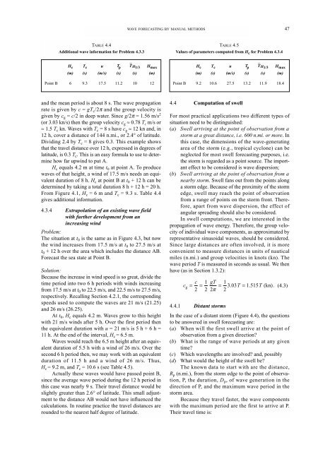
TABLE 4.4<br />
Additional wave information for Problem 4.3.3<br />
Hc Tc u Tp –<br />
TH1/3 Hmax (m) (s) (m/s) (s) (s) (m)<br />
Point B 6 9.3 17.5 11.2 10 12<br />
and the mean period is about 8 s. The wave propagation<br />
rate is given by c = gT c/2π and the group velocity is<br />
given by c g = c/2 in deep water. Since g/2π = 1.56 m/s 2<br />
(or 3.03 kn/s) then the group velocity c g ≈ 0.78 T c m/s or<br />
≈ 1.5 T c kn. Waves with T c = 8 s have c g ≈ 12 kn and, in<br />
12 h, cover a distance of 144 n.mi., or 2.4° of latitude.<br />
Dividing 2.4 by T c = 8 gives 0.3. This example shows<br />
that the travel distance over 12 h, expressed in degrees of<br />
latitude, is 0.3 T c. This is an easy formula to use to determine<br />
how far upwind to put A.<br />
H c equals 4.2 m at time t 0 at point A. To produce<br />
waves of that height, a wind of 17.5 m/s needs an equivalent<br />
duration of 8 h. H c at point B at t 0 + 12 h can be<br />
determined by taking a total duration 8 h + 12 h = 20 h.<br />
From Figure 4.1, H c = 6 m and T c = 9.3 s. Table 4.4<br />
gives additional information.<br />
4.3.4 Extrapolation of an existing wave field<br />
with further development from an<br />
increasing wind<br />
Problem:<br />
The situation at t0 is the same as in Figure 4.3, but now<br />
the wind increases from 17.5 m/s at t0 to 27.5 m/s at<br />
t0 + 12 h over the area which includes the distance AB.<br />
Forecast the sea state at Point B.<br />
Solution:<br />
Because the increase in wind speed is so great, divide the<br />
time period into two 6 h periods with winds increasing<br />
from 17.5 m/s at t 0 to 22.5 m/s, and 22.5 m/s to 27.5 m/s,<br />
respectively. Recalling Section 4.2.1, the corresponding<br />
speeds used to compute the waves are 21 m/s (21.25)<br />
and 26 m/s (26.25).<br />
At t 0, H c equals 4.2 m. Waves grow to this height<br />
with 21 m/s winds after 5 h. Over the first period then<br />
the equivalent duration with u = 21 m/s is 5 h + 6 h =<br />
11 h. At the end of the interval, H c = 6.5 m.<br />
Waves would reach the 6.5 m height after an equivalent<br />
duration of 5.5 h with a wind of 26 m/s. Over the<br />
second 6 h period then, we may work with an equivalent<br />
duration of 11.5 h and a wind of 26 m/s. Thus,<br />
H c = 9.2 m, and T c = 10.6 s (see Table 4.5).<br />
Actually these waves would have passed point B,<br />
since the average wave period during the 12 h period in<br />
this case was nearly 9 s. Their travel distance would be<br />
slightly greater than 2.6° of latitude. This small adjustment<br />
to the distance AB would not have influenced the<br />
calculations. In routine practice the travel distances are<br />
rounded to the nearest half degree of latitude.<br />
<strong>WAVE</strong> <strong>FORECASTING</strong> BY MANUAL METHODS 47<br />
TABLE 4.5<br />
Values of parameters computed from Hc for Problem 4.3.4<br />
4.4 Computation of swell<br />
For most practical applications two different types of<br />
situation need to be distinguished:<br />
(a) Swell arriving at the point of observation from a<br />
storm at a great distance, i.e. 600 n.mi. or more. In<br />
this case, the dimensions of the wave-generating<br />
area of the storm (e.g., tropical cyclone) can be<br />
neglected for most swell forecasting purposes, i.e.<br />
the storm is regarded as a point source. The important<br />
effect to be considered is wave dispersion;<br />
(b) Swell arriving at the point of observation from a<br />
nearby storm. Swell fans out from the points along<br />
a storm edge. Because of the proximity of the storm<br />
edge, swell may reach the point of observation<br />
from a range of points on the storm front. Therefore,<br />
apart from wave dispersion, the effect of<br />
angular spreading should also be considered.<br />
In swell computations, we are interested in the<br />
propagation of wave energy. Therefore, the group velocity<br />
of individual wave components, as approximated by<br />
representative sinusoidal waves, should be considered.<br />
Since large distances are often involved, it is more<br />
convenient to measure distances in units of nautical<br />
miles (n.mi.) and group velocities in knots (kn). The<br />
wave period T is measured in seconds as usual. We then<br />
have (as in Section 1.3.2):<br />
c<br />
g<br />
Hc Tc u Tp –<br />
TH1/3 Hmax (m) (s) (m/s) (s) (s) (m)<br />
Point B 9.2 10.6 27.5 13.2 11.9 18.4<br />
c 1 gT 1<br />
= = = 3. 03T = 1. 515T<br />
(kn).<br />
2 2 2π<br />
2<br />
(4.3)<br />
4.4.1 Distant storms<br />
In the case of a distant storm (Figure 4.4), the questions<br />
to be answered in swell forecasting are:<br />
(a) When will the first swell arrive at the point of<br />
observation from a given direction?<br />
(b) What is the range of wave periods at any given<br />
time?<br />
(c) Which wavelengths are involved? and, possibly<br />
(d) What would the height of the swell be?<br />
The known data to start with are the distance,<br />
Rp (n.mi.), from the storm edge to the point of observation,<br />
P, the duration, Dp, of wave generation in the<br />
direction of P, and the maximum wave period in the<br />
storm area.<br />
Because they travel faster, the wave components<br />
with the maximum period are the first to arrive at P.<br />
Their travel time is:


