GUIDE WAVE ANALYSIS AND FORECASTING - WMO
GUIDE WAVE ANALYSIS AND FORECASTING - WMO
GUIDE WAVE ANALYSIS AND FORECASTING - WMO
You also want an ePaper? Increase the reach of your titles
YUMPU automatically turns print PDFs into web optimized ePapers that Google loves.
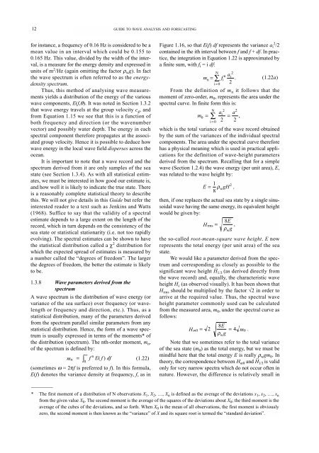
12<br />
for instance, a frequency of 0.16 Hz is considered to be a<br />
mean value in an interval which could be 0.155 to<br />
0.165 Hz. This value, divided by the width of the interval,<br />
is a measure for the energy density and expressed in<br />
units of m 2 /Hz (again omitting the factor ρ wg). In fact<br />
the wave spectrum is often referred to as the energydensity<br />
spectrum.<br />
Thus, this method of analysing wave measurements<br />
yields a distribution of the energy of the various<br />
wave components, E(f,θ). It was noted in Section 1.3.2<br />
that wave energy travels at the group velocity c g, and<br />
from Equation 1.15 we see that this is a function of<br />
both frequency and direction (or the wavenumber<br />
vector) and possibly water depth. The energy in each<br />
spectral component therefore propagates at the associated<br />
group velocity. Hence it is possible to deduce how<br />
wave energy in the local wave field disperses across the<br />
ocean.<br />
It is important to note that a wave record and the<br />
spectrum derived from it are only samples of the sea<br />
state (see Section 1.3.4). As with all statistical estimates,<br />
we must be interested in how good our estimate is,<br />
and how well it is likely to indicate the true state. There<br />
is a reasonably complete statistical theory to describe<br />
this. We will not give details in this Guide but refer the<br />
interested reader to a text such as Jenkins and Watts<br />
(1968). Suffice to say that the validity of a spectral<br />
estimate depends to a large extent on the length of the<br />
record, which in turn depends on the consistency of the<br />
sea state or statistical stationarity (i.e. not too rapidly<br />
evolving). The spectral estimates can be shown to have<br />
the statistical distribution called a χ 2 distribution for<br />
which the expected spread of estimates is measured by<br />
a number called the “degrees of freedom”. The larger<br />
the degrees of freedom, the better the estimate is likely<br />
to be.<br />
1.3.8 Wave parameters derived from the<br />
spectrum<br />
A wave spectrum is the distribution of wave energy (or<br />
variance of the sea surface) over frequency (or wavelength<br />
or frequency and direction, etc.). Thus, as a<br />
statistical distribution, many of the parameters derived<br />
from the spectrum parallel similar parameters from any<br />
statistical distribution. Hence, the form of a wave spectrum<br />
is usually expressed in terms of the moments* of<br />
the distribution (spectrum). The nth-order moment, mn, of the spectrum is defined by:<br />
n<br />
m n = f E( f ) df (1.22)<br />
(sometimes ω = 2πf is preferred to f). In this formula,<br />
E(f) denotes the variance density at frequency, f, as in<br />
∞<br />
∫0 _________<br />
<strong>GUIDE</strong> TO <strong>WAVE</strong> <strong>ANALYSIS</strong> <strong>AND</strong> <strong>FORECASTING</strong><br />
2 Figure 1.16, so that E(f) df represents the variance ai /2<br />
contained in the ith interval between f and f + df. In practice,<br />
the integration in Equation 1.22 is approximated by<br />
a finite sum, with fi = i df:<br />
m f (1.22a)<br />
From the definition of mn it follows that the<br />
moment of zero-order, m0, represents the area under the<br />
spectral curve. In finite form this is:<br />
a<br />
n i n<br />
N 2<br />
i = ∑ .<br />
i = 0 2<br />
which is the total variance of the wave record obtained<br />
by the sum of the variances of the individual spectral<br />
components. The area under the spectral curve therefore<br />
has a physical meaning which is used in practical applications<br />
for the definition of wave-height parameters<br />
derived from the spectrum. Recalling that for a simple<br />
wave (Section 1.2.4) the wave energy (per unit area), E,<br />
was related to the wave height by:<br />
then, if one replaces the actual sea state by a single sinusoidal<br />
wave having the same energy, its equivalent height<br />
would be given by:<br />
8E<br />
Hrms<br />
= ,<br />
ρ g<br />
the so-called root-mean-square wave height. E now<br />
represents the total energy (per unit area) of the sea<br />
state.<br />
We would like a parameter derived from the spectrum<br />
and corresponding as closely as possible to the<br />
significant wave height H – 1/3 (as derived directly from<br />
the wave record) and, equally, the characteristic wave<br />
height H c (as observed visually). It has been shown that<br />
H rms should be multiplied by the factor √2 in order to<br />
arrive at the required value. Thus, the spectral wave<br />
height parameter commonly used can be calculated<br />
from the measured area, m 0, under the spectral curve as<br />
follows:<br />
H<br />
m<br />
0<br />
N<br />
a a<br />
= ∑ =<br />
2 2<br />
i ,<br />
i = 0<br />
E = gH ,<br />
1 2<br />
ρw 8<br />
8E<br />
= 2 = 4<br />
m .<br />
m0<br />
0<br />
ρwg Note that we sometimes refer to the total variance<br />
of the sea state (m 0) as the total energy, but we must be<br />
mindful here that the total energy E is really ρ wgm 0. In<br />
theory, the correspondence between H m0 and H – 1/3 is valid<br />
only for very narrow spectra which do not occur often in<br />
nature. However, the difference is relatively small in<br />
* The first moment of a distribution of N observations X 1, X 2, …, X n is defined as the average of the deviations x 1, x 2, …, x n<br />
from the given value X 0. The second moment is the average of the squares of the deviations about X 0; the third moment is the<br />
average of the cubes of the deviations, and so forth. When X 0 is the mean of all observations, the first moment is obviously<br />
zero, the second moment is then known as the “variance” of X and its square root is termed the “standard deviation”.<br />
2<br />
w<br />
2


