Proceedings of the 2009 northeastern recreation research symposium
Proceedings of the 2009 northeastern recreation research symposium
Proceedings of the 2009 northeastern recreation research symposium

Create successful ePaper yourself
Turn your PDF publications into a flip-book with our unique Google optimized e-Paper software.
Table 1.—Viewshed results for all 16 points with qrea <strong>of</strong> visible land cover types in hectares<br />
Point Developed Agriculture Shrubland/<br />
Woodland<br />
Forested<br />
Land<br />
Water Wetland<br />
Barren<br />
Land<br />
1 3.60 0.09 0.00 245.73 0.00 0.00 0.00 249.42<br />
2 0.18 0.09 0.00 236.72 0.00 0.00 0.00 236.99<br />
3 0.00 0.18 0.00 228.89 0.00 0.00 0.00 229.07<br />
4 0.00 0.18 0.00 260.40 0.00 0.00 0.09 260.67<br />
5 0.00 0.00 0.00 343.96 0.00 0.36 0.00 344.32<br />
6 0.00 0.00 0.00 708.10 0.00 0.18 0.00 708.28<br />
7 0.00 19.63 3.24 879.36 0.00 0.09 0.00 902.32<br />
8 0.00 11.71 13.06 3667.18 0.00 11.89 0.00 3703.84<br />
9 3.69 1969.51 124.17 12,465.60 89.50 44.48 1.17 14,698.12<br />
10 0.54 72.93 29.71 7298.44 0.81 3.51 1.71 7407.65<br />
11 9.54 110.66 53.40 12,233.20 1.53 0.63 26.20 12,435.16<br />
12 3.51 136.78 44.03 10,906.60 0.72 1.08 55.65 11,148.37<br />
13 0.00 3.24 3.51 697.65 0.00 0.00 0.00 704.4<br />
14 0.00 71.31 22.87 3914.08 0.18 5.49 0.27 4014.2<br />
15 9.09 92.29 28.54 6323.63 0.00 1.44 6.75 6461.74<br />
16 12.52 647.95 83.11 11,658.20 47.63 3.06 13.42 12,465.89<br />
Figure 4.—GIS map showing viewshed from point 16.<br />
3.3 Scenic Beauty Modeling<br />
<strong>Proceedings</strong> <strong>of</strong> <strong>the</strong> <strong>2009</strong> Nor<strong>the</strong>astern Recreation Research Symposium GTR-NRS-P-66<br />
Total<br />
Th e independent variables (i.e., <strong>the</strong> land cover types)<br />
considered for <strong>the</strong> regression had high levels <strong>of</strong><br />
correlation. As a result, only <strong>the</strong> forest, agriculture,<br />
and nonvegetated land (combined barren land and<br />
developed area) variables were used. Tables 2 and<br />
3 show <strong>the</strong> regression estimates <strong>of</strong> scenic beauty<br />
for each month. Th e regression for September was<br />
not signifi cant, but <strong>the</strong> regression for October was<br />
signifi cant at <strong>the</strong> 5 percent level <strong>of</strong> signifi cance, and<br />
<strong>the</strong> variables in <strong>the</strong> model explained 43 percent <strong>of</strong> <strong>the</strong><br />
variation in scenic beauty values. Only <strong>the</strong> variable<br />
“forest” was signifi cant at <strong>the</strong> 5 percent level. Th e<br />
positive sign indicated that increasing <strong>the</strong> total forest<br />
area would increase <strong>the</strong> value <strong>of</strong> <strong>the</strong> scenic beauty in late<br />
fall. Fur<strong>the</strong>rmore, <strong>the</strong> negative sign <strong>of</strong> <strong>the</strong> nonvegetated<br />
areas (i.e., barren and developed) indicates an inverse<br />
relationship with scenic beauty values when o<strong>the</strong>r<br />
factors are held constant.<br />
Forest cover had a signifi cantly positive relationship<br />
with scenic beauty for October but not for September,<br />
implying that scenery in <strong>the</strong> area is more beautiful in<br />
October than in September. Although <strong>the</strong> area <strong>of</strong> land<br />
184