A Semi-Implicit, Three-Dimensional Model for Estuarine ... - USGS

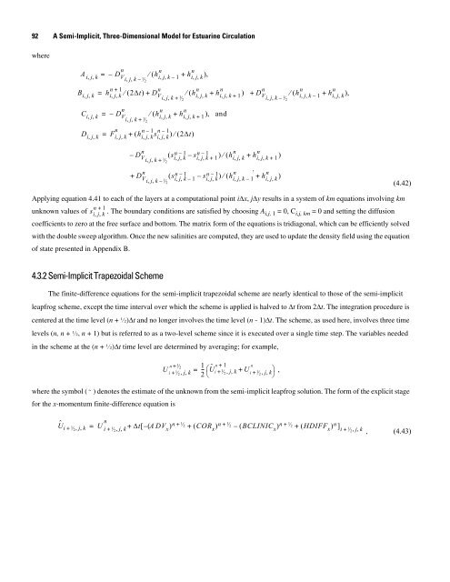
92 A Semi-Implicit, Three-Dimensional Model for Estuarine Circulation
where
A i, j, k
Bi, j, k
Ci, j, k
Di, j, k
=
n
– DV i, j, k – 1⁄ 2
n + 1
n
= hi, j, k⁄
( 2Δt ) + DV , ,
=
=
n
– DVi , j, k+ 1⁄ 2
n
Fi, j, k
n
n
⁄ ( hi, j, k – 1 + hijk , , ) ,
i j k+ 1⁄ 2
n n
n
⁄ ( hijk , , + hi, j, k+ 1)
+ DV , ,
n n
⁄ ( hi, j, k+
hijk , , + 1)
, and
n – 1 n – 1
+ ( hi, j, ksijk
, , ) ⁄ ( 2Δt )
–
+
n
DV n
DV ijk , , + 1⁄ 2
ijk , , – 1⁄ 2
i j k – 1⁄ 2
sn – 1
i, j, k sn – 1 n n
( – i, j, k + 1)
⁄ ( hijk , , + hi, j, k+ 1)
sn – 1
ijk , , – 1 sn – 1 n · n
( – i, j, k)
⁄ ( hi, j, k– 1 + hi, j, k)
n
n
⁄ ( hi, j, k – 1 + hi, j, k)
,
Applying equation 4.41 to each of the layers at a computational point iΔx, jΔy results in a system of km equations involving km
n + 1
unknown values of sijk , , . The boundary conditions are satisfied by choosing Ai,j, 1 = 0, Ci,j, km = 0 and setting the diffusion
coefficients to zero at the free surface and bottom. The matrix form of the equations is tridiagonal, which can be efficiently solved
with the double sweep algorithm. Once the new salinities are computed, they are used to update the density field using the equation
of state presented in Appendix B.
4.3.2 Semi-Implicit Trapezoidal Scheme
The finite-difference equations for the semi-implicit trapezoidal scheme are nearly identical to those of the semi-implicit
leapfrog scheme, except the time interval over which the scheme is applied is halved to Δt from 2Δt. The integration procedure is
centered at the time level (n + ½)Δt and no longer involves the time level (n - 1)Δt. The scheme, as used here, involves three time
levels (n, n + ½, n + 1) but is referred to as a two-level scheme since it is executed over a single time step. The variables needed
in the scheme at the (n + ½)Δt time level are determined by averaging; for example,
+ ⁄ 1 n + 1
n
--
+ , j, k=
⎛Ũi+ 1⁄ 2 , j, k+
U i 1 ⎞
2
+ ⁄ 2 , j, k ,
⎝ ⎠
n 1
2
U i 1⁄ 2
where the symbol ( ˜ ) denotes the estimate of the unknown from the semi-implicit leapfrog solution. The form of the explicit stage
for the x-momentum finite-difference equation is
Ûi + 1⁄ 2,
jk , = U i 1⁄ 2
n
+ , j, k Δt ( ADVx) n + 1⁄ 2 ( CORx) n 1
[ –
+
+ ⁄ 2 ( BCLINICx) n 1
+ – + ⁄ 2 + HDIFFx ( ) n ] i 1⁄ 2
(4.42)
+ , jk , , (4.43)