A Semi-Implicit, Three-Dimensional Model for Estuarine ... - USGS

72 A Semi-Implicit, Three-Dimensional Model for Estuarine Circulation
4.2.1 Two-Level Semi-Implicit Scheme
The two-level semi-implicit scheme closely resembles the iterative scheme first published by Abbott and Ionescu (1967) and
later used by Verwey (1971) in a model for the Danish Hydraulic Institute. The scheme here is most similar to the version of the
Abbott-Ionescu scheme described by Cunge and others (1980, p. 97−98). One change in the scheme here is in the manner in which
the system of finite-difference equations are formed for each time step. The momentum equations are substituted into the continuity
equations so that a linear system of equations is formed involving only the unknown water surface elevations {ζ i }. This reduces
the size of the matrix to be solved to half the size of one involving both dependent variables. For typical 1-D problems the savings
in storage space for the reduced matrix generally is not important, but the savings for 3-D problems can be significant.
The equations are solved by using separate explicit and implicit stages to keep the computer code modular. In a solution for
one dimensional flow with homogeneous density, only the advection term in the momentum equation is treated explicitly. Owing
to the staggered grid, the continuity and momentum equations are applied to different control volumes shifted one-half cell relative
to one another. Continuity is applied at the ζ-points and momentum is applied at the U-points.
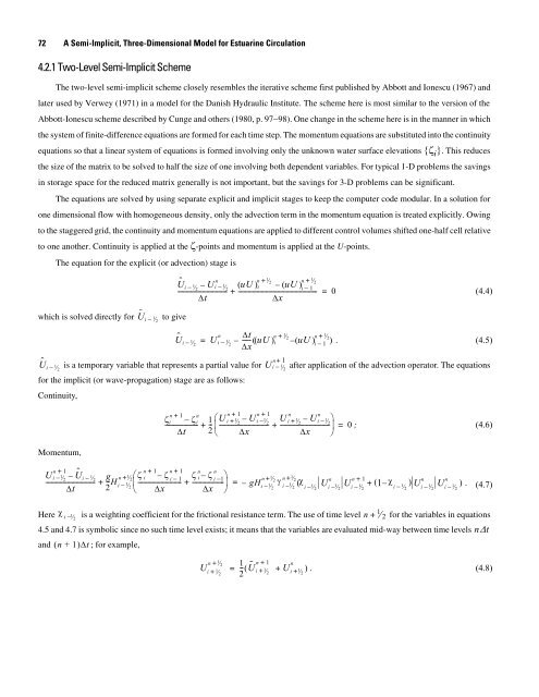
The equation for the explicit (or advection) stage is
which is solved directly for Ûi – 1⁄ to give
2
Ûi – 1⁄ 2
+ ⁄
+ ⁄
n
n 1
2
n 1
2
Ûi – 1⁄ – U 2 i – 1⁄ ( uU ) 2
i – ( uU ) i – 1
--------------------------------- + ----------------------------------------------------- = 0
(4.4)
Δt
Δx
n
Ûi – 1⁄ = U 2 i – 1⁄ 2
– Δt n + 1⁄ 2 n + 1⁄ 2
------ ( uU ) i – ( uU ) i – 1 ) .
Δx
n 1
is a temporary variable that represents a partial value for U i – 1⁄ 2
for the implicit (or wave-propagation) stage are as follows:
Continuity,
Momentum,
(4.5)
+ after application of the advection operator. The equations
n + 1 n
ζi – ζ i 1
---------------------- --
Δt 2
U n + 1 n + 1
i + 1⁄ – U 2 i – 1⁄ 2
----------------------------------
Δx
U n
n
⎛ i + 1⁄ – U 2 i – 1⁄ ⎞
2
+ ⎜ + ---------------------------------- ⎟ = 0 ; (4.6)
⎝ Δx ⎠
n + 1
n 1 n 1 n n
U i – 1⁄ – Ûi 1
2 – ⁄ 2 g n + 1⁄ ⎛ζ 2 i – ζ i 1
--------------------------------- --H
– ζ i – ζ i – ⎞ 1
n + 1⁄ 2 n + 1
+ i – 1⁄ ⎜---------------------------- + --------------------- ⎟ = – gH γ ⁄ 2 χ
2
i – 1⁄ 2 i – 1⁄ 2 i – 1⁄ 2
U n n + 1
i – 1 Ui 1 ⁄ 2 – ⁄ 2
Δt
Here χ i 1⁄ 2
2
+
+
⎝ Δx Δx ⎠
1 χ n n
( + ( – i – 1 )U ⁄ 2 i – 1 Ui 1 ⁄ 2 – ) .
⁄ (4.7)
2
– is a weighting coefficient for the frictional resistance term. The use of time level n + 1
2 for the variables in equations
4.5 and 4.7 is symbolic since no such time level exists; it means that the variables are evaluated mid-way between time levels nΔt
and ( n + 1)Δt
; for example,
+ ⁄ 1 n + 1 n
= -- ( Ũ i + 1
2 2 ⁄ + Ui + 1⁄ ) .
(4.8)
2
n 1
2
Ui + 1⁄ 2
⁄